<?xml version="1.0" encoding="utf-8"?><feed xmlns="http://www.w3.org/2005/Atom" ><generator uri="https://jekyllrb.com/" version="3.9.5">Jekyll</generator><link href="/feed.xml" rel="self" type="application/atom+xml" /><link href="/" rel="alternate" type="text/html" /><updated>2024-02-28T22:09:40+00:00</updated><id>/feed.xml</id><title type="html">Capsules Bot</title><subtitle>Exploring autonomous systems, robotics and mapping.</subtitle><author><name>Pavlo Bashmakov</name></author><entry><title type="html">Lidar odometry smoothing using ES EKF and KissICP for Ouster sensors with IMUs</title><link href="/blog/2024/02/05/esekf-smoothing-ouster-lidar-with-imu-using-kiss.html" rel="alternate" type="text/html" title="Lidar odometry smoothing using ES EKF and KissICP for Ouster sensors with IMUs" /><published>2024-02-05T08:00:00+00:00</published><updated>2024-02-05T08:00:00+00:00</updated><id>/blog/2024/02/05/esekf-smoothing-ouster-lidar-with-imu-using-kiss</id><content type="html" xml:base="/blog/2024/02/05/esekf-smoothing-ouster-lidar-with-imu-using-kiss.html"><![CDATA[<p>In this post I’ve explored the possibility of improving the KissICP trajectory output for Ouster Lidars using the sensor’s embedded IMUs. On some  environments ES EKF filtering together with KissICP made the <em>10%</em> decrease in the ATE for high resolution 128 beam sensors but on other environments with lower resolution 32 beam sensors it showed <em>50%</em> decrease in ATE compared to ground truth. ES EKF filter formulation and experiments described with references, source code and CLI tools for visualizations that may be used to replicate and test approaches on any Ouster’s Lidar pcap/bag raw data recordings.</p>

<h2 id="motivation-and-related-works">Motivation and Related works</h2>

<p>Since Ouster Lidar has an embedded IMU with time synchronization with lidar scans it should be beneficial to utilize it for Lidar based odometry and, possibly, reduce the drift, avoid system degradation on feature-less environments and improve results in fast movement scenarios.</p>

<p>As a good starting point to review the current state of Lidar based odometry and different approaches you can check this <em>“LiDAR Odometry Survey <a href="#references">[1]</a>“</em>.</p>

<p>In my experiment I will extend on the KissICP <a href="#references">[2]</a> implementation since it’s already tested with Ouster sensors and it’s SDK <a href="#references">[3]</a>. The main test dataset used for experiments is Newer College Dataset 2021 extension <a href="#references">[4]</a> with OS-0 128 beam sensor and latest Ouster sensors sample raw data recordings <a href="#references">[5]</a></p>

<h2 id="overall-system-description">Overall system description</h2>

<p>The input to the system is an Ouster lidar raw sensor data in the form of UDP packets payload from pcap/bag container.</p>

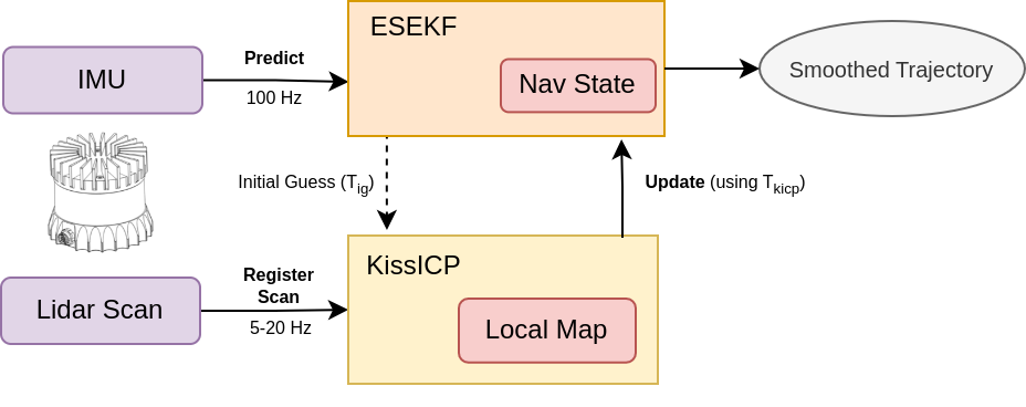
<p>ES EKF performs state prediction and error-state tracking on every incoming IMU measurement. When the new scan is available KissICP registers it, optionally using the ES EKF state as the initial pose guess, and the resulting pose used for the ES EKF update step. The output of the system is the ES EKF state which is the smoothed trajectory, see <em>Fig. 1</em> below.</p>

<div class="fig figcenter fighighlight">
  <img src="/imgs/esekf_smoothing_ouster_lidar/esekf-kissicp.png" />
  <div class="margin:0">Fig 1. Ouster lidar odometry with KissICP + ESEKF trajectory smoothing (lously coupled)</div>
</div>

<p><em>NOTE:</em> Even though the <em>imu packets</em> and <em>lidar packets</em> is the Ouster wire data format and the pipeline works with live sensors too one should make additional efforts to tune the setup for the specific system performance which depends on machine setup (compute, memory, network), sensor resolution (32, 64 or 128 beams), KissICP parameters (internal map size, downsampling ratios, etc.) and sensor configuration (lidar mode, lidar profile, etc).</p>

<h2 id="es-ekf-error-state-extended-kalman-filter-formulation">ES EKF: Error-state Extended Kalman Filter formulation</h2>

<p>The main effect of the ES EKF contribution to the pipeline is to integrate the available IMU information and fuse it with the KissICP trajectory output while also providing the better initial guess for the point cloud registration step.</p>

<p>The exposition of the ES EKF below is very brief and more like to provide the overall structure of what is inside with the references to other sources with fully detailed derivations, possible modifications to update steps, etc. I heavily relied on the work “Quaternion kinematics for the error-state Kalman filter” by Joan Sola <a href="#references">[6]</a> where the Error-state EKF derivations and formulations were cleanly presented for the quaternions but could be easily adopted for the exponential representations.</p>

<p>Other important sources: in-depth IMU mechanisations for low-cost sensors could be found in <a href="#references">[7]</a>, Kalman filters modular design approaches <a href="#references">[8]</a>, multi sensor data fusion <a href="#references">[9]</a> and useful background theory and results on Lie Groups for 3D <a href="#references">[10, 11, 12]</a></p>

<h1 id="predict-step-using-new-imu-measurement">Predict step using new IMU measurement</h1>

<p>The nominal filter state is defined as the following:</p>

\[\boldsymbol{x} = \{ \boldsymbol{t}, \boldsymbol{v}, \boldsymbol{R}, \boldsymbol{b_g}, \boldsymbol{b_a} \}\]

<p>where $\boldsymbol{t},\boldsymbol{v} \in \mathbb{R}^{3}$ are the position and velocity in global frame, $\boldsymbol{R} \in SO(3)$ (or alternatively $\boldsymbol{q} \in \mathbb{H}$ can be used) is a rotation in global frame (as a rotation matrix or quaternion) and $\boldsymbol{b_g}, \boldsymbol{b_a} \in \mathbb{R}^{3}$ are gyroscope and accelerometer biases to be estimated.</p>

<p>Nominal state discrete-time kinematics, i.e. predict step that happens on every new IMU measurement:</p>

\[\begin{aligned}
  \boldsymbol{\tilde{t}_k} &amp; = t_{k-1} + v_{k-1} \Delta{t} + \frac{1}{2}(R_{k-1}(a_k - b_{a,k-1}) + \boldsymbol{g})\Delta{t}^2 \\
  \boldsymbol{\tilde{v}_k} &amp; = v_{k-1} + (R_{k-1}(a_k - b_{a,k-1}) + \boldsymbol{g})\Delta{t} \\
  \boldsymbol{\tilde{R}_k} &amp; = R_{k-1} Exp((\omega_k - b_{g,k-1})\Delta{t})) \\
  \boldsymbol{\tilde{b}_{g,k}} &amp; = b_{g,k-1} \\
  \boldsymbol{\tilde{b}_{a,k}} &amp; = b_{a,k-1}
\end{aligned}\]

<p>Let’s define the nominal state evolved during the IMU prediction step as $\boldsymbol{\tilde{x}_k}$.</p>

<p>The error-state is defined as following:</p>

\[\boldsymbol{\delta{x}} = \{ \boldsymbol{\delta{t}}, \boldsymbol{\delta{v}}, \boldsymbol{\delta{\phi}}, \boldsymbol{\delta{b_g}}, \boldsymbol{\delta{b_a}} \}\]

<p>where $\boldsymbol{\delta{t}}, \boldsymbol{\delta{v}}, \boldsymbol{\delta{\phi}} \in \mathbb{R}^3$ is the position, velocity and rotation errors, $\boldsymbol{\delta{b_g}}, \boldsymbol{\delta{b_a}} \in \mathbb{R}^3$ is the bias errors of gyroscope and accelerometer.</p>

<p>Error-state is evolving together with a nominal state in-between the update steps on IMU measurements and its kinematics in discrete-time:</p>

\[\begin{aligned}

\boldsymbol{\delta{t}_k} &amp; = \delta{t}_{k-1} + \delta{v}_{k-1} \Delta{t} \\
\boldsymbol{\delta{v}_k} &amp; = \delta{v}_{k-1} + (-R_{k-1}[\mathbf{a}_k - b_{a, k-1}]_{\times}\delta{\phi}_{k-1} - R_{k-1}\delta{b_{a,k-1}})\Delta{t} + \mathbf{v_i} \\
\boldsymbol{\delta{\phi}_k} &amp; = Exp((\mathbf{\omega}_k - b_{g, k-1})\Delta{t})^{T}\delta{\phi}_{k-1} - \delta{b_{g, k-1}}\Delta{t} + \mathbf{\phi_i} \\
\boldsymbol{\delta{b_{g, k}}} &amp; = \delta{b_{g, k-1}} + \mathbf{\omega_i} \\
\boldsymbol{\delta{b_{a, k}}} &amp; = \delta{b_{a, k-1}} + \mathbf{a_i}

\end{aligned}\]

<p>where $\mathbf{v_i}, \mathbf{\phi_i}, \mathbf{\omega_i}$ and $\mathbf{a_i}$ are the random impulses modeled as white Gaussian processes. Integrating the corresponding covariances of accelerometer/gyriscope biases and random walks we obtain the noise covariance matrices:</p>

\[\begin{aligned}

\boldsymbol{V_i} &amp; = \sigma_{a_n}^2 \Delta{t}^{2} \boldsymbol{I} \\
\boldsymbol{\Phi_i} &amp; = \sigma_{\omega_n}^2 \Delta{t}^{2} \boldsymbol{I} \\
\boldsymbol{\Omega_i} &amp; = \sigma_{\omega_w}^2 \Delta{t} \boldsymbol{I} \\
\boldsymbol{A_i} &amp; = \sigma_{a_w}^2 \Delta{t} \boldsymbol{I}

\end{aligned}\]

<p>Introducing the input signal vector, from IMU measurement, and random process impulses vector as $\boldsymbol{u_k} = [a_k, \omega_k]^T$, $\boldsymbol{i} = [\boldsymbol{v_i}, \boldsymbol{\phi_i}, \boldsymbol{a_i}, \boldsymbol{\omega_i}]^T$ the error-state system can be written as:</p>

\[\boldsymbol{\delta{x}_k} \leftarrow f(\boldsymbol{\tilde{x}_{k-1}}, \boldsymbol{\delta{x_{k-1}}}, \boldsymbol{u_k}, \boldsymbol{i}) = F_x(\boldsymbol{x_{k-1}}, \boldsymbol{u_k}) \delta{x} + F_i \boldsymbol{i}\]

<p>ES EKF predict step equations then (for error-state mean $\boldsymbol{\delta_x} \in \mathbb{R}^{15}$ and process covariance $\boldsymbol{P} \in \mathbb{R}^{15 \times 15}$ estimates):</p>

\[\begin{aligned}
\boldsymbol{\delta{x}_k} &amp; = F_x(\boldsymbol{x_{k-1}}, \boldsymbol{u_k}) \delta{x} \\
\boldsymbol{P_k} &amp; = F_x \boldsymbol{P_{k-1}} F_{x}^T + F_i \boldsymbol{Q_i} F_{i}^T
\end{aligned}\]

<p>In expressions above $F_x$ is a Jacobian of the error-state transition function at the current point $\boldsymbol{x}_k, \boldsymbol{u_k}$ and can be written as:</p>

\[F_x = \frac{\partial{f}}{\partial{\delta{x}}}\bigg|_{x_{k-1}, u_k} = \begin{bmatrix}  \boldsymbol{I} &amp;&amp; \boldsymbol{I} \Delta{t} &amp;&amp; 0 &amp;&amp; 0 &amp;&amp; 0 \\
0 &amp;&amp; \boldsymbol{I} &amp;&amp; -R_{k-1}[\mathbf{a}_k - b_{a, k-1}]_{\times}\Delta{t} &amp;&amp; 0 &amp;&amp; - R_{k-1}\Delta{t} \\
0 &amp;&amp; 0 &amp;&amp; Exp((\mathbf{\omega}_k - b_{g, k-1})\Delta{t})^{T} &amp;&amp; - \boldsymbol{I}\Delta{t} &amp;&amp; 0 \\
0 &amp;&amp; 0 &amp;&amp; 0 &amp;&amp; \boldsymbol{I} &amp;&amp; 0 \\
0 &amp;&amp; 0 &amp;&amp; 0 &amp;&amp; 0 &amp;&amp; \boldsymbol{I} \end{bmatrix}\]

<p>and $F_i$ is a Jacobian with respect to random impulses $\boldsymbol{i}$ which can be written as:</p>

\[F_i = \frac{\partial{f}}{\partial{\boldsymbol{i}}}\bigg|_{x_{k-1}, u_k} = \begin{bmatrix} 0 &amp;&amp; 0 &amp;&amp; 0 &amp;&amp; 0 \\
\boldsymbol{I} &amp;&amp; 0 &amp;&amp; 0 &amp;&amp; 0 \\
0 &amp;&amp; \boldsymbol{I} &amp;&amp; 0 &amp;&amp; 0 \\
0 &amp;&amp; 0 &amp;&amp; \boldsymbol{I} &amp;&amp; 0 \\
0 &amp;&amp; 0 &amp;&amp; 0 &amp;&amp; \boldsymbol{I} \end{bmatrix}
\,, \quad
Q_i = \begin{bmatrix}
\boldsymbol{V_i} &amp;&amp; 0 &amp;&amp; 0 &amp;&amp; 0 \\
0 &amp;&amp; \boldsymbol{\Phi_i} &amp;&amp; 0 &amp;&amp; 0 \\
0 &amp;&amp; 0 &amp;&amp; \boldsymbol{\Omega_i} &amp;&amp; 0 \\
0 &amp;&amp; 0 &amp;&amp; 0 &amp;&amp; \boldsymbol{A_i} \end{bmatrix}\]

<h1 id="update-step-using-kissicp-pose">Update step using KissICP pose</h1>

<p>KissICP registers every lidar frame, with optional initial guess pose obtained from the ES EKF filter, and returns the new system pose $z_k = T_{kicp, k} = [ R_{kicp, k} \, \vert \, t_{kicp, k} ]$ which then used in the update state of the filter.</p>

<p>The measurement model $h(\hat{x}_k)$ that is using the best true-state at the time of update $\hat{x}_k = \tilde{x} \oplus \delta{x}_k$ is:</p>

\[h(\hat{x}_k) = h(\tilde{x} \oplus \delta{x}_k) = [ \tilde{R}_k Exp(\delta{\phi}_k) \, \vert \, \tilde{t}_k + \delta{t}_k  ]\]

<p>The Jacobian $H$ of the measurement model with respect to the error-state $\delta{x}$ is defined as:</p>

\[H = \frac{\partial{h}}{\partial{\delta{x}}} \bigg|_x = \begin{bmatrix}
\boldsymbol{I} &amp;&amp; 0 &amp;&amp; 0 &amp;&amp; 0 &amp;&amp; 0 \\
0 &amp;&amp; 0 &amp;&amp; \boldsymbol{I} &amp;&amp; 0 &amp;&amp; 0
\end{bmatrix} \quad \in \mathbb{R}^{6 \times 15}\]

<p>The measurement residual thus is:</p>

\[y_k = z_k \ominus h(\hat{x}) = \begin{bmatrix}
t_{kicp,k} - \tilde{t}_k - \delta{t}_k \\
Log(Exp(\delta{\phi}_k)^T \tilde{R}_k^T R_{kicp, k})
\end{bmatrix} \, \in \mathbb{R}^{1 \times 6}\]

<p>Now the complete set of equations for the ES EKF update step can be expressed as:</p>

\[\begin{aligned}
S &amp; = H \boldsymbol{P}_{k-1} H^T + \boldsymbol{V} \\
K &amp; = \boldsymbol{P}_{k-1} H^T S^{-1} \\
\delta{x}_k &amp; \leftarrow K y_k \\
\boldsymbol{P}_k &amp; \leftarrow (\boldsymbol{I} - K H) \boldsymbol{P}_{k-1}
\end{aligned}\]

<p>where $\boldsymbol{V} \in \mathbb{R}^{6 \times 6}$ is the measurement error covariances of pose translation and pose rotation, which highly depends on the sensor used and it’s accuracy specs.</p>

<h1 id="inject-the-error-into-nominal-state-and-reset-the-error-state">Inject the error into nominal state and reset the error-state</h1>

<p>After we’ve got a KissICP pose $T_{kicp,k}$ estimate and updated the error-state mean $\delta{x}_k$ and covariance $P_k$ we need to incorporate the error-state into nominal state $\boldsymbol{x}_k = \tilde{x}_k \oplus \delta{x}_k$, or in expanded form:</p>

\[\begin{aligned}
\boldsymbol{t}_k &amp; = \tilde{t}_k + \delta{t}_k \\
\boldsymbol{v}_k &amp; = \tilde{v}_k + \delta{v}_k \\
\boldsymbol{R}_k &amp; = \tilde{R}_k Exp(\delta{\phi}_k) \\
\boldsymbol{b}_{g,k} &amp; = \tilde{b}_{g,k} + \delta{b}_{g,k} \\
\boldsymbol{b}_{a,k} &amp; = \tilde{b}_{a,k} + \delta{b}_{a,k}
\end{aligned}\]

<p>Then we reset the error-state $\delta{x} \leftarrow 0$ and ready to receive the new IMU measurements and execute predict step and so on.</p>

<p>Covariance $\boldsymbol{P}$ maybe left unchanged on the reset step or corrected to decrease the long-term error and odometry drift, please refer to <a href="#references">[6], eqns 285-287</a> for details and derivations of such covariance correction.</p>

<h2 id="experimental-results">Experimental results</h2>

<p>The ES EKF implementation was done as part of the <code class="language-plaintext highlighter-rouge">ptudes ekf-bench</code> (<a href="https://github.com/bexcite/ptudes-lab">Point eTudes</a>) playground with metrics visualization, ground truth comparison (with ATE calculations) and point cloud visualization (with <a href="/blog/2023/12/04/point-etudes-lab-flyby.html"><code class="language-plaintext highlighter-rouge">flyby</code> viz</a> for qualitative reviews). Newer College Dataset 2021 <a href="#references">[4]</a> extension was used to compare the results with ground truth.</p>

<h3 id="simulated-imu-data-or-direct-gt-poses">Simulated IMU data or direct GT poses</h3>

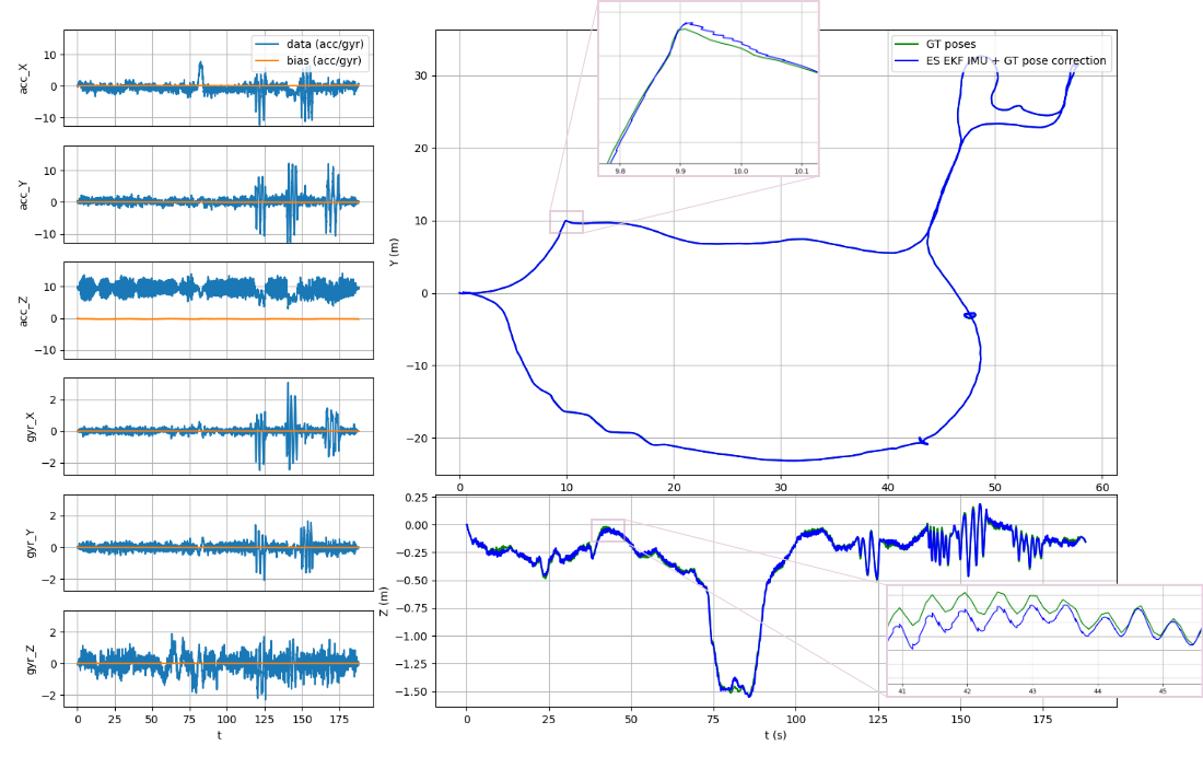
<p>The basic operation of ES EKF was validated with simulated IMU with/without noise that can be compared to the dead reckoning INS in the absence of the accelerometer/gyroscope noise and biases and using the ground truth poses as a correction input to check the filter convergence (see <code class="language-plaintext highlighter-rouge">ptudes ekf-bench sim</code> and <code class="language-plaintext highlighter-rouge">ptudes ekf-bench nc</code> commands correspondingly).</p>

<div class="fig figcenter fighighlight">
  <img src="/imgs/esekf_smoothing_ouster_lidar/esekf-nc-hard-result.png" />
  <div class="margin:0">Fig 2. ESEKF run on Newer <i>College collection1/quad-hard</i> sequence with direct GT pose correction (<code>ptudes ekf-bench nc</code>)</div>
</div>

<p>The ES EKF performance of tracking the IMU inputs with direct ground truth poses as an update on the <em>collection1/quad-hard</em> sequence of the Newer College 2021 Dataset shown on Fig. 2 above, the Average Trajectory Errors (ATE) for position and rotation resulting in <code class="language-plaintext highlighter-rouge">0.0007 m</code> and <code class="language-plaintext highlighter-rouge">0.0004 deg</code> correspondingly (see <a href="#references">[13]</a> for ATE calculations details).</p>

<h3 id="ouster-lidar-data-with-imu">Ouster Lidar data with IMU</h3>

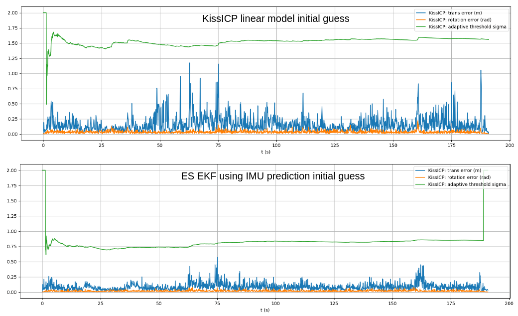
<p>The full pipeline with Ouster Lidar data and its IMU data streams was implemented in the <code class="language-plaintext highlighter-rouge">ptudes ekf-bench ouster</code> command that accepts Ouster raw data recordings in pcap/bag formats. Additionally ground truth can be provided in Newer College Dataset format using <code class="language-plaintext highlighter-rouge">--gt-file</code> param which is used only to compare the results and compare the graphs of trajectories (using <code class="language-plaintext highlighter-rouge">--plot graphs</code>) and the adaptive threshold of the KissICP registration together with it’s corrected pose translation and rotation components (the less value of sigma of the adaptive threshold the more “confident” KissICP registration is for the particular scan, see <a href="#references">[2]</a> for KissICP algorithm details).</p>

<p>Tests was performed using sequences <em>quad-easy/medium/hard</em> and <em>stairs</em> from <em>collection1</em> and <em>park0</em>, <em>park1</em> and <em>cloister0</em> from collection2, with/without using ES EKF imu prediction guess for KissICP registration. Additionally the tests with manually reduced beams number (32,64 and 128) on <em>quad-medium</em> sequence was compared. In majority of test cases the ES EKF imu predicted initial guess improved the resulting pose with reduced ATE errors, the most significant gains observed on 32 beams cases and harder movements like <em>quad-hard</em> or <em>stairs</em> sequences, see Table 1. for full results.</p>

<table>
  <thead>
    <tr>
      <th>Sequence name</th>
      <th>Lidar Beams</th>
      <th>KissICP range (m) min - max</th>
      <th>ATE (deg) / trans (m)</th>
      <th>ATE rot (deg) / trans (m) w imu prediction</th>
    </tr>
  </thead>
  <tbody>
    <tr>
      <td>nc-quad-easy</td>
      <td>128</td>
      <td>1 - 35</td>
      <td><strong>0.0256</strong> / <strong>0.1383</strong></td>
      <td>0.0282 / 0.1834</td>
    </tr>
    <tr>
      <td>nc-quad-easy</td>
      <td>64</td>
      <td>1 - 35</td>
      <td><strong>0.0318</strong> / <strong>0.0978</strong></td>
      <td>0.0791 / 0.8966</td>
    </tr>
    <tr>
      <td>nc-quad-easy</td>
      <td>32</td>
      <td>1 - 35</td>
      <td>1.0932 / 7.6802</td>
      <td><strong>0.3722</strong> / <strong>6.1207</strong></td>
    </tr>
    <tr>
      <td>nc-quad-medium</td>
      <td>128</td>
      <td>1 - 35</td>
      <td>0.0715 / 0.3817</td>
      <td><strong>0.0434</strong> / <strong>0.1121</strong></td>
    </tr>
    <tr>
      <td>nc-quad-medium</td>
      <td>64</td>
      <td>1 - 35</td>
      <td><strong>0.1884</strong> / <strong>1.5852</strong></td>
      <td>0.2190 / 1.8996</td>
    </tr>
    <tr>
      <td>nc-quad-medium</td>
      <td>32</td>
      <td>1 - 35</td>
      <td>5.7766 / 36.7806</td>
      <td><strong>0.5252</strong> / <strong>6.1870</strong></td>
    </tr>
    <tr>
      <td>nc-quad-hard</td>
      <td>128</td>
      <td>1 - 35</td>
      <td>0.1072 / <strong>0.3465</strong></td>
      <td><strong>0.0954</strong> / 0.3582</td>
    </tr>
    <tr>
      <td>nc-quad-hard</td>
      <td>64</td>
      <td>1 - 35</td>
      <td>0.3947 / 5.5880</td>
      <td><strong>0.1045</strong> / <strong>0.3003</strong></td>
    </tr>
    <tr>
      <td>nc-quad-hard</td>
      <td>32</td>
      <td>1 - 35</td>
      <td>1.8676 / 22.8112</td>
      <td><strong>0.3869</strong> / <strong>6.9918</strong></td>
    </tr>
    <tr>
      <td>nc-stairs</td>
      <td>128</td>
      <td>1 - 17</td>
      <td>1.1885 / 0.3389</td>
      <td><strong>0.3467</strong> / <strong>0.1182</strong></td>
    </tr>
    <tr>
      <td>nc-park0</td>
      <td>128</td>
      <td>1 - 35</td>
      <td><strong>0.5302</strong> / <strong>24.3595</strong></td>
      <td>0.5379 / 24.5963</td>
    </tr>
    <tr>
      <td>nc-park1</td>
      <td>128</td>
      <td>1 - 35</td>
      <td>0.1151 / 8.3812</td>
      <td><strong>0.0593</strong> / <strong>2.4570</strong></td>
    </tr>
    <tr>
      <td>nc-cloister0</td>
      <td>128</td>
      <td>1 - 17</td>
      <td>0.3031 / 6.0323</td>
      <td><strong>0.3014</strong> / <strong>5.7621</strong></td>
    </tr>
    <tr>
      <td>nc-cloister0</td>
      <td>128</td>
      <td>1 - 35</td>
      <td><strong>0.1598</strong> / <strong>2.9759</strong></td>
      <td>0.2001 / 3.8562</td>
    </tr>
  </tbody>
</table>

<p><em>Table 1</em>. Test results using ES EKF pipeline with IMU predicted initial guess vs linear KissICP initial guess (baseline).</p>

<p>The adaptive threshold value of KissICP tracks in most cases lower with IMU prediction pose guess (correspondingly the difference to corrected pose after ICP iterations is also lower), see Fig 3.</p>

<div class="fig figcenter fighighlight">
  <img src="/imgs/esekf_smoothing_ouster_lidar/esekf-kissicp-threshold.png" />
  <div class="margin:0">Fig 3. Adaptive Threshold Sigma with KissICP initial guess vs ESEKF IMU prediction initial guess</div>
</div>

<h2 id="source-code-and-cli-to-run-it-with-ouster-lidar-sensors-data">Source code and CLI to run it with Ouster Lidar sensors data</h2>

<p>The ES EKF + KissICP trajectory smoothing developed as part of <code class="language-plaintext highlighter-rouge">ptudes ekf-bench</code> (<a href="https://github.com/bexcite/ptudes-lab">Point eTudes</a>) playground and can be installed from PyPi (python 3.7-3.11, Win/Mac/Linux supported):</p>

<div class="language-plaintext highlighter-rouge"><div class="highlight"><pre class="highlight"><code>pip install ptudes-lab
</code></pre></div></div>

<p>For example to run on the <em>cloister0</em> sequence bag from Newer College Dataset and visualize the result you can run:</p>

<div class="language-plaintext highlighter-rouge"><div class="highlight"><pre class="highlight"><code># process raw Ouster packets from .bag and run KissICP + ES EKF smoothing and save traj poses
ptudes ekf-bench ouster ./newer-college/2021-ouster-os0-128-alphasense/collection2/2021-12-02-10-15-59_0-cloister.bag \
  --save-nc-gt-poses cloister0-traj.csv

# visualize the part of the bag in a flyby tool
ptudes flyby ./newer-college/2021-ouster-os0-128-alphasense/collection2/2021-12-02-10-15-59_0-cloister.bag \
  --nc-gt-poses cloister0-traj.csv \
  --start-scan 400 \
  --end-scan 800
</code></pre></div></div>

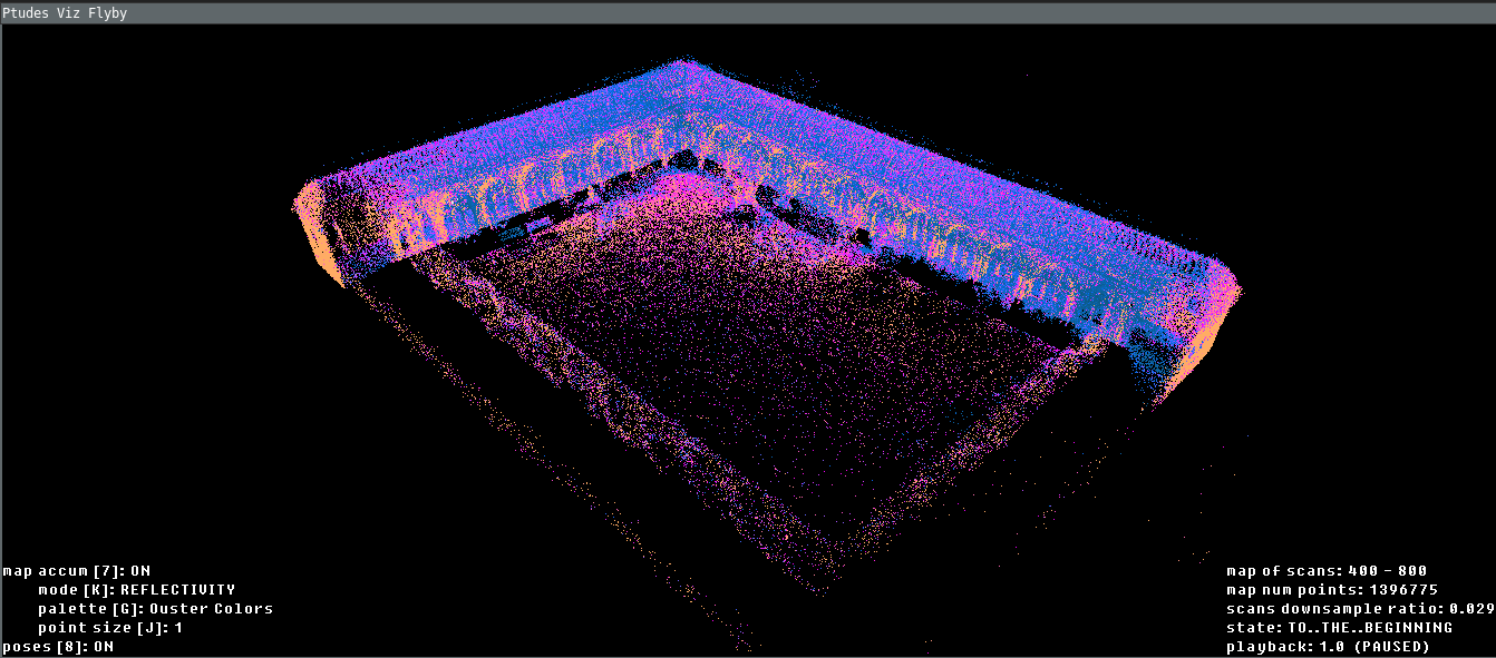
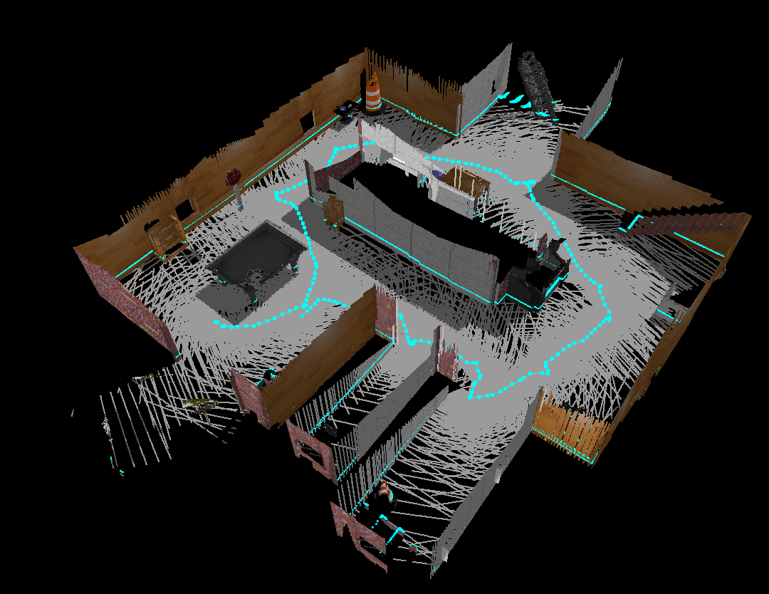
<p>With the viz result shown below:</p>

<div class="fig figcenter fighighlight">
  <img src="/imgs/esekf_smoothing_ouster_lidar/esekf-cloister0-400-800.png" />
  <div class="margin:0">Fig 4. <code>ptudes flyby</code> over the <i>cloister0</i> sequence scans <i>400-800</i></div>
</div>

<p>Simulated IMU runs, ES EKF with real IMU topic but ground truth poses as a correction or comparing various trajectories with ATE scores calculated use <code class="language-plaintext highlighter-rouge">ptudes ekf-bench sim</code>, <code class="language-plaintext highlighter-rouge">ptudes ekf-bench nc</code> and <code class="language-plaintext highlighter-rouge">ptudes ekf-bench cmp</code> correspondingly.</p>

<p>To get the overall statistic of the IMU/Lidar scans from the <code class="language-plaintext highlighter-rouge">pcap/bag</code> you can use <code class="language-plaintext highlighter-rouge">ptudes stat</code> which may <em>hint</em> you the optimal value of <code class="language-plaintext highlighter-rouge">--kiss-min-range/--kiss-max-range</code> params to use:</p>
<div class="language-plaintext highlighter-rouge"><div class="highlight"><pre class="highlight"><code>ptudes stat ./newer-college/2021-ouster-os0-128-alphasense/collection2/2021-12-02-10-15-59_0-cloister.bag -t 0
</code></pre></div></div>

<p>With an output:</p>
<div class="language-plaintext highlighter-rouge"><div class="highlight"><pre class="highlight"><code>StreamStatsTracker[dt: 186.5307 s, imus: 18652, scans: 1866]:
  range_mean: 4.457 m,
  range_std: 4.139 m (s3 span: [0.234 - 16.874 m])
  range min max: 0.234 - 220.712 m
  acc_mean: [-0.18887646  0.41429864  9.72023424] m/s^2
  acc_std: [0.63840631 0.59747534 2.30738675]
  gyr_mean: [-0.01103721 -0.00591911  0.07017822] rad/s
  gyr_std: [0.09329166 0.14244756 0.34110766]
Gravity vector estimation:  [-0.01940998  0.0425756   0.99890469]
</code></pre></div></div>

<p><em>NOTE</em>: estimated gravity vector doesn’t account for the movements and valid only when the lidar was stationary during the recording.</p>

<p>Checkout the previous blog post on (<a href="/blog/2023/12/04/point-etudes-lab-flyby.html">Point eTudes</a>) for other nits.</p>

<h2 id="possible-future-work-and-experiments">Possible future work and experiments</h2>

<p>ES EKF is a common building block in state-of-the art and recent efforts in Lidar Inertial Odometry like FAST-LIO2 <a href="#references">[15]</a>, LIO-EKF <a href="#references">[14]</a>, SR-LIO and many others. However, as mentioned above algorithms are tightly coupled LIO systems and they usually has much better performance than loosely-coupled counterparts, so it’s worth considering them for further adoption and experimenting to get the better Lidar-Inertial odometry.</p>

<p><a name="references"></a></p>

<h2 id="references">References</h2>

<ol>
  <li>Lee, Dongjae, et al. <a href="https://arxiv.org/pdf/2312.17487.pdf">“LiDAR Odometry Survey: Recent Advancements and Remaining Challenges.”</a> (2023)</li>
  <li>Vizzo, Ignacio, et al. <a href="https://arxiv.org/pdf/2209.15397.pdf">“Kiss-icp: In defense of point-to-point icp–simple, accurate, and robust registration if done the right way.”</a> (2023)</li>
  <li>Ouster SDK: C++/Python sensor driver and tools, CLI, PointViz, etc. <a href="https://github.com/ouster-lidar/ouster_example">“GitHub”</a></li>
  <li>Zhang, Lintong, et al. <a href="https://arxiv.org/pdf/2112.08854.pdf">“Multi-camera lidar inertial extension to the newer college dataset.”</a> (2021).</li>
  <li>Ouster sensor raw sample data <a href="https://static.ouster.dev/sensor-docs/#sample-data">“Sensor Docs/Sample Data</a></li>
  <li>Sola, Joan. <a href="https://arxiv.org/pdf/1711.02508.pdf">“Quaternion kinematics for the error-state Kalman filter.”</a> (2017).</li>
  <li>Shin, Eun-Hwan. <a href="https://www.ucalgary.ca/engo_webdocs/NES/05.20219.EHShin.pdf">“Estimation techniques for low-cost inertial navigation.”</a> (2005).</li>
  <li>Maley, James, and DEVCOM Army Research Laboratory. <a href="https://apps.dtic.mil/sti/trecms/pdf/AD1126850.pdf">“A Modular Approach to Kalman Filter Design and Analysis.”</a> (2021).</li>
  <li>Durrant-Whyte, Hugh. <a href="https://citeseerx.ist.psu.edu/document?repid=rep1&amp;type=pdf&amp;doi=6998134026e385977f75ec9243dfc2af924688b0">“Multi Sensor Data Fusion.”</a> (2001).</li>
  <li>Eade, Ethan. <a href="https://ethaneade.org/lie.pdf">“Lie groups for 2d and 3d transformations.”</a> (2017).</li>
  <li>Sola, Joan, Jeremie Deray, and Dinesh Atchuthan. <a href="https://arxiv.org/pdf/1812.01537.pdf">“A micro Lie theory for state estimation in robotics.”</a> (2018).</li>
  <li>Daniel Lawrence Lu, <a href="https://daniel.lawrence.lu/blog/y2021m09d08/">“SE(3) constraints for robotics”</a> (2021).</li>
  <li>Zhang, Zichao, and Davide Scaramuzza. <a href="https://www.zora.uzh.ch/id/eprint/175991/1/IROS18_Zhang.pdf">“A tutorial on quantitative trajectory evaluation for visual (-inertial) odometry.”</a> (2018).</li>
  <li>Wu, Yibin, et al. <a href="https://arxiv.org/pdf/2311.09887.pdf">“Lio-ekf: High frequency lidar-inertial odometry using extended kalman filters.”</a> (2023).</li>
  <li>Xu, Wei, et al. <a href="https://arxiv.org/pdf/2107.06829.pdf">“Fast-lio2: Fast direct lidar-inertial odometry.”</a> (2022).</li>
  <li>Yuan, Zikang, et al. <a href="">“Sr-lio: Lidar-inertial odometry with sweep reconstruction.”</a> (2022).</li>
</ol>]]></content><author><name>Pavlo Bashmakov</name></author><category term="blog" /><summary type="html"><![CDATA[In this post I’ve explored the possibility of improving the KissICP trajectory output for Ouster Lidars using the sensor’s embedded IMUs. On some environments ES EKF filtering together with KissICP made the 10% decrease in the ATE for high resolution 128 beam sensors but on other environments with lower resolution 32 beam sensors it showed 50% decrease in ATE compared to ground truth. ES EKF filter formulation and experiments described with references, source code and CLI tools for visualizations that may be used to replicate and test approaches on any Ouster’s Lidar pcap/bag raw data recordings.]]></summary></entry><entry><title type="html">P(oint) (e)Tudes: Lidar odometry, SLAM and visualization tools</title><link href="/blog/2023/12/04/point-etudes-lab-flyby.html" rel="alternate" type="text/html" title="P(oint) (e)Tudes: Lidar odometry, SLAM and visualization tools" /><published>2023-12-04T08:00:00+00:00</published><updated>2023-12-04T08:00:00+00:00</updated><id>/blog/2023/12/04/point-etudes-lab-flyby</id><content type="html" xml:base="/blog/2023/12/04/point-etudes-lab-flyby.html"><![CDATA[<p>I’ve started the <code class="language-plaintext highlighter-rouge">ptudes</code> (<a href="https://github.com/bexcite/ptudes-lab">Point eTudes</a>) playground as a place to easily run and replicate experiments with lidar based odometry, slam and mapping.</p>

<p>It’s heavily based on my latest work on <a href="https://github.com/ouster-lidar/ouster_example">Ouster SDK</a> which was in the areas related to (the list is far from exhaustive):</p>

<ul>
  <li>raw sensor pcap reader integration to <a href="https://github.com/PRBonn/kiss-icp">KISS-ICP</a>, so one can easily get poses per every scan with a <code class="language-plaintext highlighter-rouge">kiss_icp_pipeline --deskew ouster.pcap</code> command.</li>
  <li><a href="https://github.com/ouster-lidar/ouster_example/blob/master/python/src/ouster/viz/core.py">Ouster SDK Viz</a> – 3D point cloud visualizer that drives all visualizers of <code class="language-plaintext highlighter-rouge">ouster-cli * viz</code> commands (OpenGL/C++/Python).</li>
  <li><code class="language-plaintext highlighter-rouge">ouster.sdk.pose_util</code> with linear <code class="language-plaintext highlighter-rouge">SE(3)</code> continuous-time trajectory interpolations and other point cloud ops like dewarping and extrinsics handling.</li>
  <li><code class="language-plaintext highlighter-rouge">ouster.viz.scans_accum.ScansAccumulator</code> to make a registered point cloud from scans + poses and display it all in <code class="language-plaintext highlighter-rouge">PointViz</code>.</li>
  <li><a href="https://github.com/ouster-lidar/ouster_example/tree/master/ouster_osf">OSF</a> - streaming based, extendable binary file format with compression for storing single/multi lidar sensor data (Flatbuffers/C++/Python).</li>
</ul>

<p>With the new <code class="language-plaintext highlighter-rouge">ptudes</code> (Point eTudes) two things are added to the above mentioned list:</p>

<ol>
  <li><code class="language-plaintext highlighter-rouge">ptudes flyby</code> - flyby 3d visualizer over the registered lidar scans with poses.</li>
</ol>

<pre><code class="language-Shell">ptudes flyby ./OS-0-128_v3.0.1_1024x10.pcap --kitti-poses ./OS-0-128_v3.0.1_poses_kitti.txt
</code></pre>

<iframe width="720" height="430" src="https://www.youtube.com/embed/NmvUkyuSK6M" frameborder="0" allow="autoplay; encrypted-media" allowfullscreen=""></iframe>
<p><em>Ouster sample data of OS-0 128 beams with KISS-ICP poses</em></p>

<ol>
  <li><code class="language-plaintext highlighter-rouge">ptudes viz</code> - visualizer of ROS BAGs with raw sensor data (i.e. <a href="https://ori-drs.github.io/newer-college-dataset/">Newer College Dataset</a>)</li>
</ol>

<pre><code class="language-Shell">ptudes viz ./2021-ouster-os0-128-alphasense/collection1/2021-07-01-10-37-38-quad-easy.bag \
    --meta ./2021-ouster-os0-128-alphasense/beam_intrinsics_os0-128.json
</code></pre>

<iframe width="720" height="430" src="https://www.youtube.com/embed/9qyVXKcG9L4" frameborder="0" allow="autoplay; encrypted-media" allowfullscreen=""></iframe>
<p><em>Newer College Dataset 2021, collection 1, quad-medium BAG</em></p>

<p>How to get the <code class="language-plaintext highlighter-rouge">ptudes</code> CLI and run examples you can find on the <a href="https://github.com/bexcite/ptudes-lab">Github project page</a>. I hope it will be valuable to other people who deal with Ouster lidar data and odometry/mapping algos.</p>]]></content><author><name>Pavlo Bashmakov</name></author><category term="blog" /><summary type="html"><![CDATA[I’ve started the ptudes (Point eTudes) playground as a place to easily run and replicate experiments with lidar based odometry, slam and mapping.]]></summary></entry><entry><title type="html">3D Reconstruction using Structure from Motion (SfM) pipeline with OpenGL visualization on C++</title><link href="/blog/2019/03/12/apolloscape-sfm.html" rel="alternate" type="text/html" title="3D Reconstruction using Structure from Motion (SfM) pipeline with OpenGL visualization on C++" /><published>2019-03-12T08:00:00+00:00</published><updated>2019-03-12T08:00:00+00:00</updated><id>/blog/2019/03/12/apolloscape-sfm</id><content type="html" xml:base="/blog/2019/03/12/apolloscape-sfm.html"><![CDATA[<p>Last year at CVPR 2018, I became interested in the Apolloscape dataset and the localization task challenge that was announced for ECCV 2018. I dived into the problem: <a href="/blog/2018/08/24/apolloscape-posenet-pytorch.html">exploring the Apolloscape dataset and using PoseNet</a> with geometric loss functions <a href="#references">[1,2]</a> for direct pose prediction from monocular images. As a result, I got more interested in geometric approaches and multi-view geometry for computer vision tasks.</p>

<p>While direct deep-learning methods somewhat works for 6DOF pose regression, they are not yet precise, and research papers increasingly use a combination of the following methods: Structure from Motion (SfM) techniques, geometric-based constraints, pose graph optimizations <a href="#references">[15]</a> and 3D maps for scene understanding, visual odometry, and SLAM tasks.</p>

<p>In this project, I explore the traditional SfM pipeline and build sparse 3D reconstruction from the Apolloscape ZPark sample dataset with simultaneous OpenGL visualization.</p>

<p>My primary goal was to learn from the first principles and implement the pipeline myself. To make SfM in production or research, you might look into available libraries: COLMAP <a href="#references">[3,4]</a>, MVE <a href="#references">[5]</a>, openMVG <a href="#references">[6]</a>, VisualSFM <a href="#references">[7]</a>, PMVS2/CMVS <a href="#references">[9]</a> and Bundler <a href="#references">[8]</a>.</p>

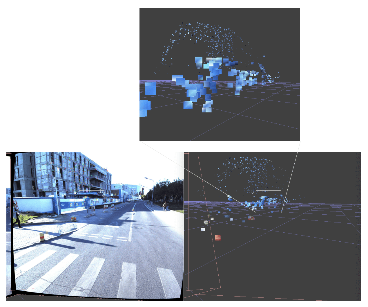
<div class="fig figcenter fighighlight">
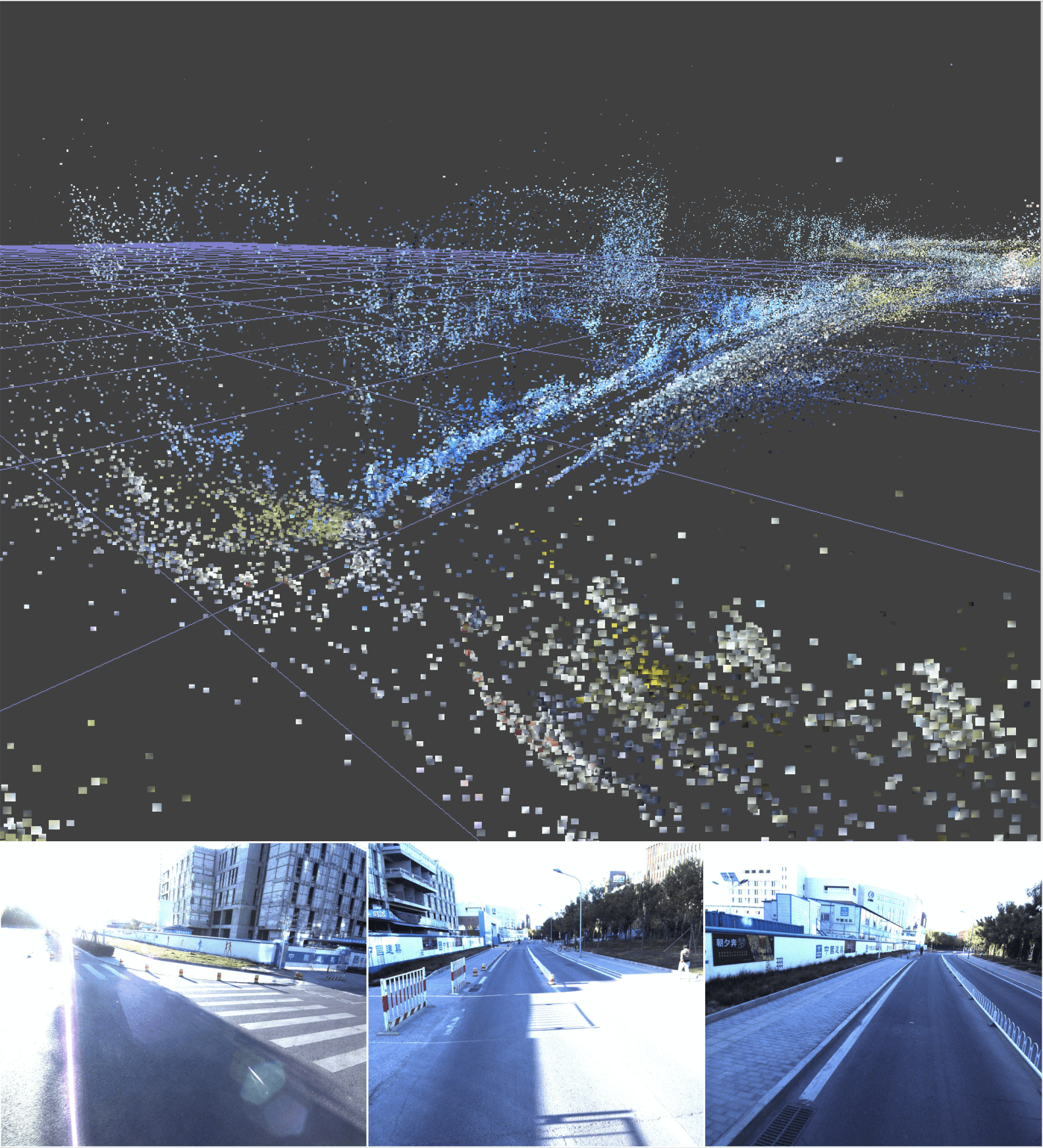
  <img src="/imgs/apolloscape_sfm/3d_recon_main.png" />
  <div class="margin:0">Structure from Motion 3D reconstruction for the Apolloscape ZPark sample dataset.</div>
</div>

<p>In this text, I use words like image, camera, or view interchangeably to relate to the same concept of an image taken with a camera in a particular location (e.g., view), and it almost always means the same in my writing and code. Sometimes it’s an image when I am preparing a dataset; a camera when I calculate the distance or projective matrix; and  a view when I am processing 3D maps and merging 3D points of different maps.</p>

<p><strong><em>NOTE</em></strong>: Code with build instructions and a reconstructed 3D map example available in my <a href="https://github.com/bexcite/apolloscape-sfm">GitHub repo</a>.</p>

<h1 id="apolloscape-dataset">Apolloscape Dataset</h1>

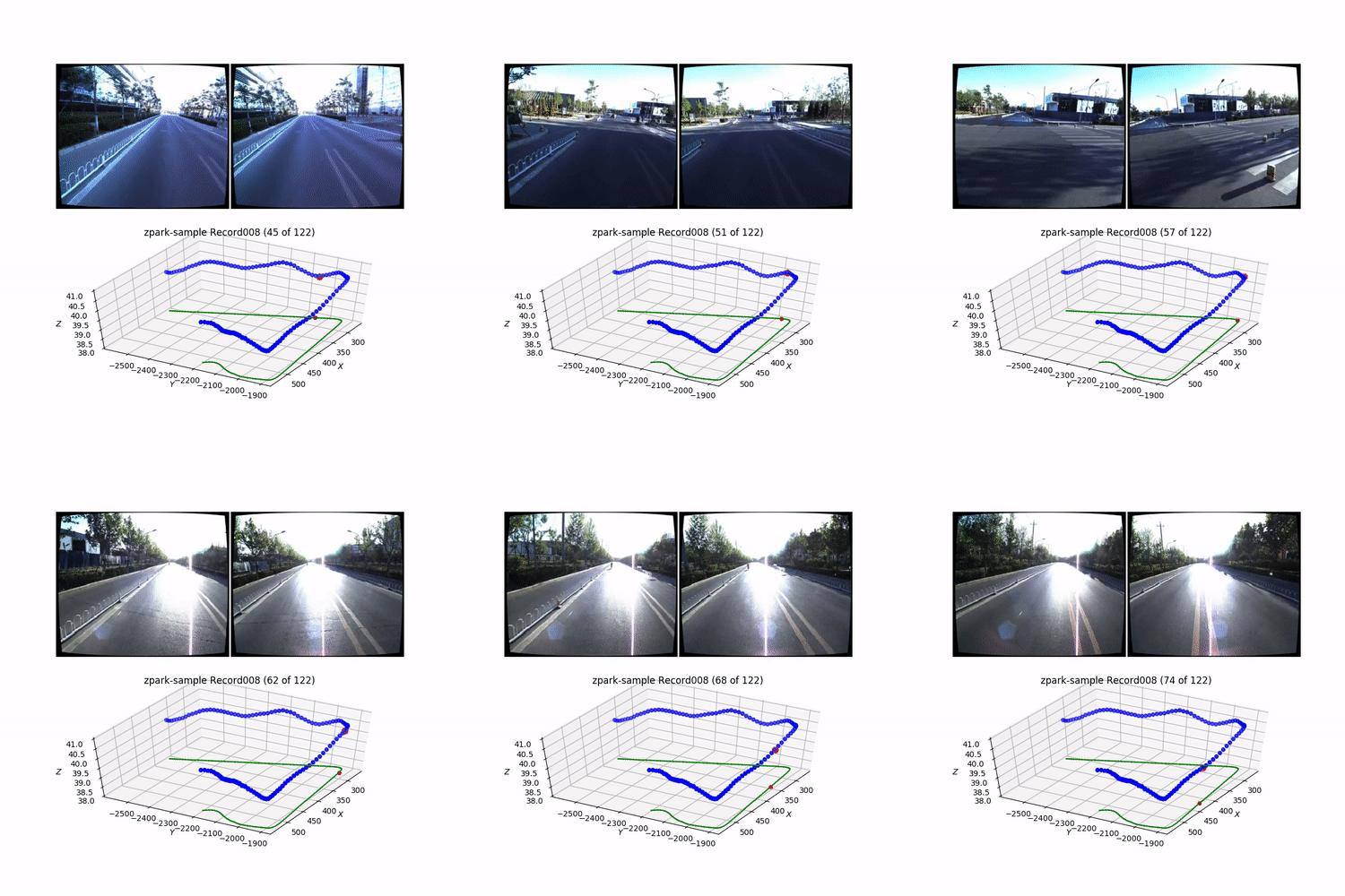
<p>In my <a href="/blog/2018/08/24/apolloscape-posenet-pytorch.html">previous article</a>, I visualize and explore the dataset. Here is the typical record (one of <code class="language-plaintext highlighter-rouge">13</code> for the ZPark sample):</p>

<div class="fig figcenter fighighlight">
  <img src="/imgs/apolloscape_sfm/video_record_008_500.gif" />
  <div class="margin:0">Visualization of Record008</div>
</div>

<p>Here is an SfM 3D reconstruction obtained from the corner shown above on a video piece:</p>

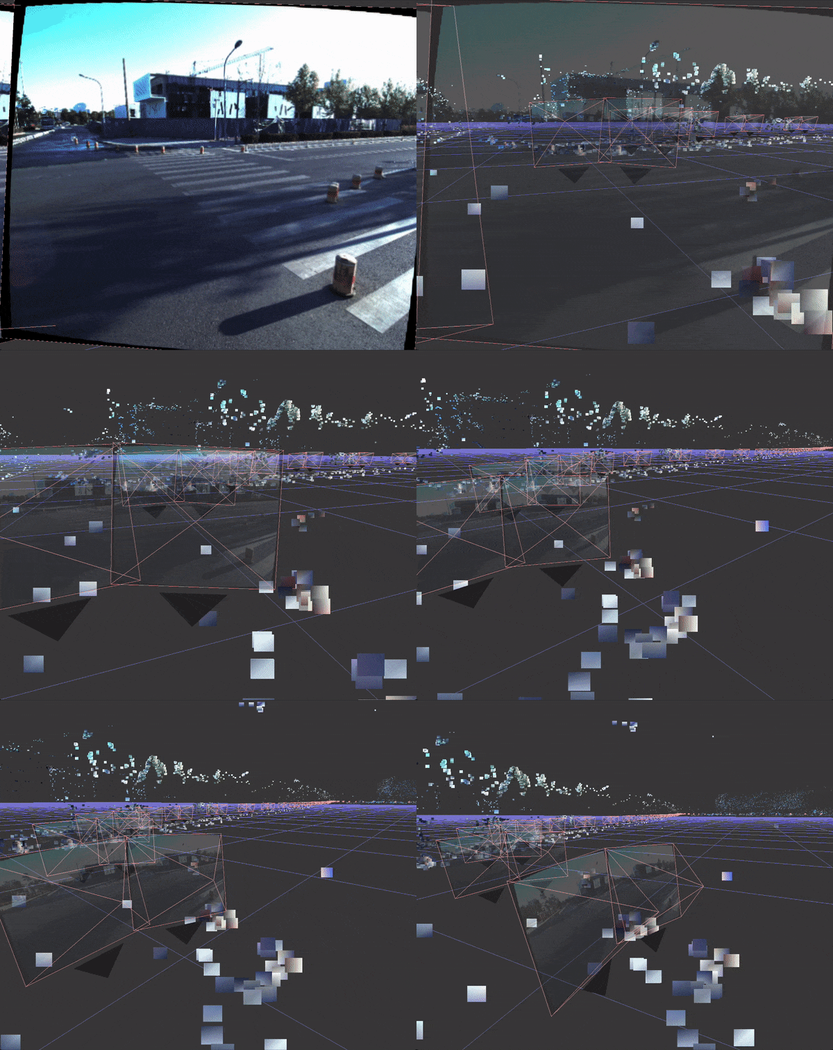
<div class="fig figcenter fighighlight">
  <img src="/imgs/apolloscape_sfm/3d_recon_8.gif" />
  <div class="margin:0">3D Reconstruction from Record008</div>
</div>

<h1 id="3d-reconstruction-results">3D Reconstruction Results</h1>

<p>In total, there <code class="language-plaintext highlighter-rouge">1,499</code> image pairs spread across <code class="language-plaintext highlighter-rouge">13</code> records in the Apolloscape ZPark sample dataset.</p>

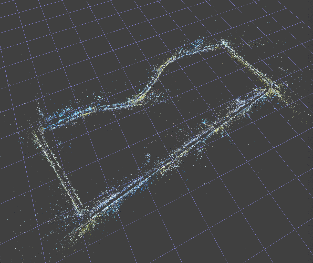
<div class="fig figcenter fighighlight">
  <img src="/imgs/apolloscape_sfm/3d_full.png" />
  <div class="margin:0">SfM 3D Reconstruction: the Apolloscape ZPark full sample dataset (2,998 images, 1.48M sparse 3D points)</div>
</div>

<p>And below is the description of the behind the scenes SfM process.</p>

<h1 id="sfm-pipeline">SfM pipeline</h1>

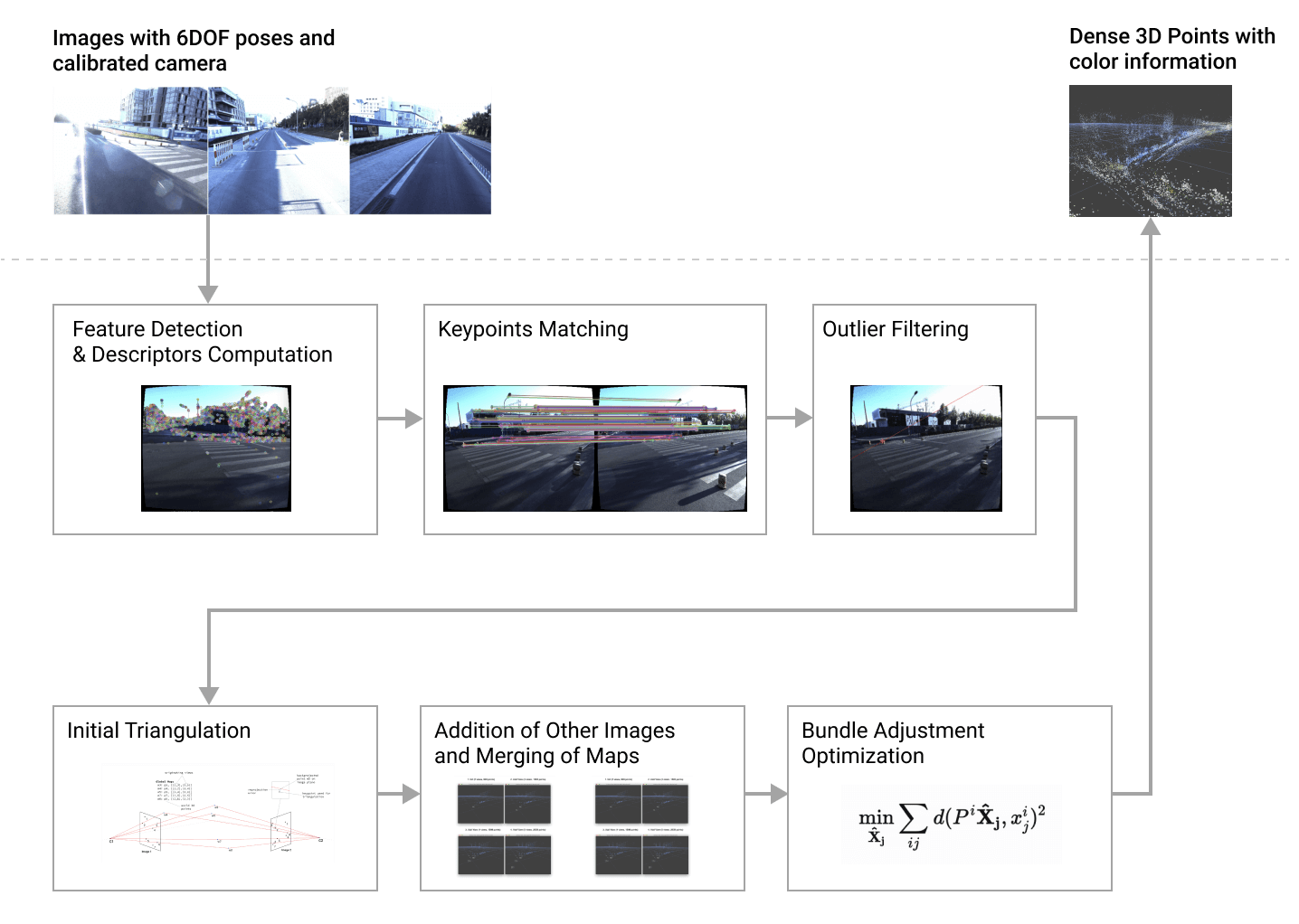
<p>The 3D reconstruction process consists of 6 major steps:</p>
<ol>
  <li>Features Detection &amp; Descriptors Computation</li>
  <li>Keypoints Matching (make image pairs, match keypoints)</li>
  <li>Outlier Filtering (via epipolar constraint)</li>
  <li>Initial Triangulation (triangulation of the best image pair)</li>
  <li>Addition of Other Images and Merging of Maps</li>
  <li>Bundle Adjustment Optimization</li>
</ol>

<div class="fig figcenter fighighlight">
  <img src="/imgs/apolloscape_sfm/sfm_3d_new.png" />
  <div class="margin:0">SfM 3D Reconstruction Pipeline</div>
</div>

<p>The described pipeline doesn’t include a couple steps from traditional SfM because we already know camera poses and need to find only world-map 3D points. These additional steps are:</p>

<ul>
  <li>2D-3D matching – finds the correspondance of 2d keypoints with already calculated 3d points, however there part of it when we find the next best view to use</li>
  <li>New image registration – estimates projection matrices based on 2d-3d matches from the previous steps</li>
  <li>Camera pose calculation – finds camera translation and rotation from the projection matrix</li>
  <li>Bundle adjustment for camera poses, together with 3D map points.</li>
</ul>

<p>The above parts can be easily added to the existing structure later when, and if, the need arises.</p>

<h2 id="features-detection--descriptors-computation">Features Detection &amp; Descriptors Computation</h2>

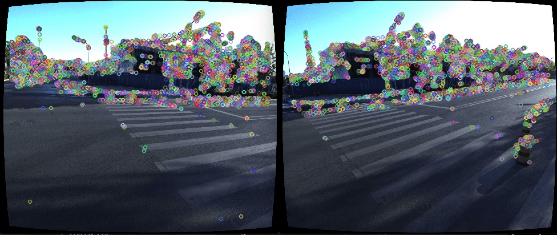
<p>First, we need to have distinctive points in the image for which we can compare and establish relationships in order to estimate image transformations or, as in the current task of reconstruction, to estimate their location in the space using multiple images.</p>

<p>There are lots of known reliable feature detectors: SURF, SIFT, ORB, BRISK, and AKAZE. I tried a couple of them from OpenCV and decided to stick with AKAZE, which gave enough points in a reasonable amount of time, with fast descriptor matching.</p>

<div class="fig figcenter fighighlight">
  <img src="/imgs/apolloscape_sfm/akaze_features.png" />
  <div class="margin:0">The AKAZE feature extractor detects, on average, 7,000 -13,000 key points from every image.</div>
</div>

<p>For further in-depth information about how different feature detectors compare, I recommend “A comparative analysis of SIFT, SURF, KAZE, AKAZE, ORB, and BRISK” <a href="#references">[10]</a>.</p>

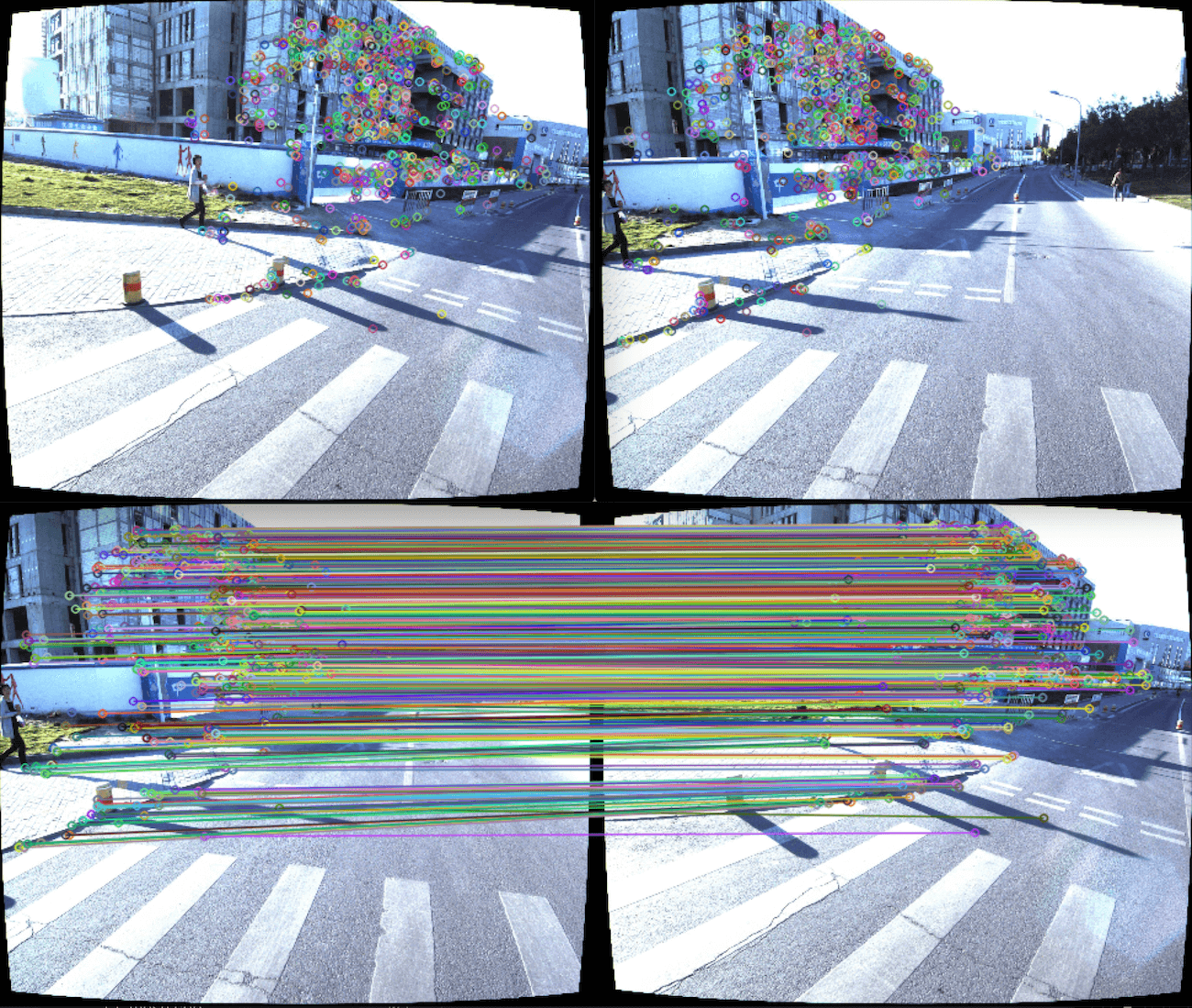
<h2 id="keypoints-matching">Keypoints Matching</h2>

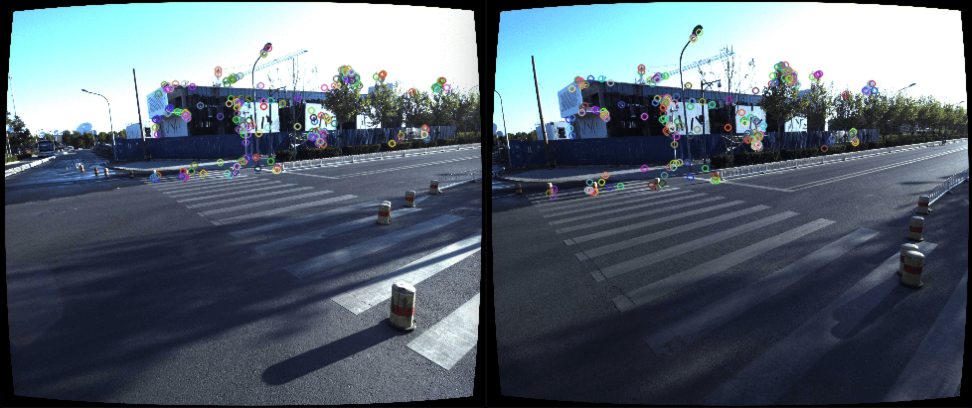
<p>The next step is to find the keypoints correspondence for every image pair. One of the common methods is to find two closest neighbors per point and compare the distance between them, aka Lowe’s ratio test <a href="#references">[11]</a>. If two closest neighbor points are located at the same distance from the original point, and they are not distinctive enough, we can skip the keypoint completely. Lowe’s paper concludes that ratio of <code class="language-plaintext highlighter-rouge">0.7</code> is a good predictor; however, in this case, I selected a ratio of <code class="language-plaintext highlighter-rouge">0.5</code> because it seemed to work better.</p>

<div class="fig figcenter fighighlight">
  <img src="/imgs/apolloscape_sfm/features_lowe_ratio.png" />
  <div class="margin:0">Correspondant AKAZE features after Lowe's ratio test (ratio 0.5). Keypoints number 224.</div>
</div>

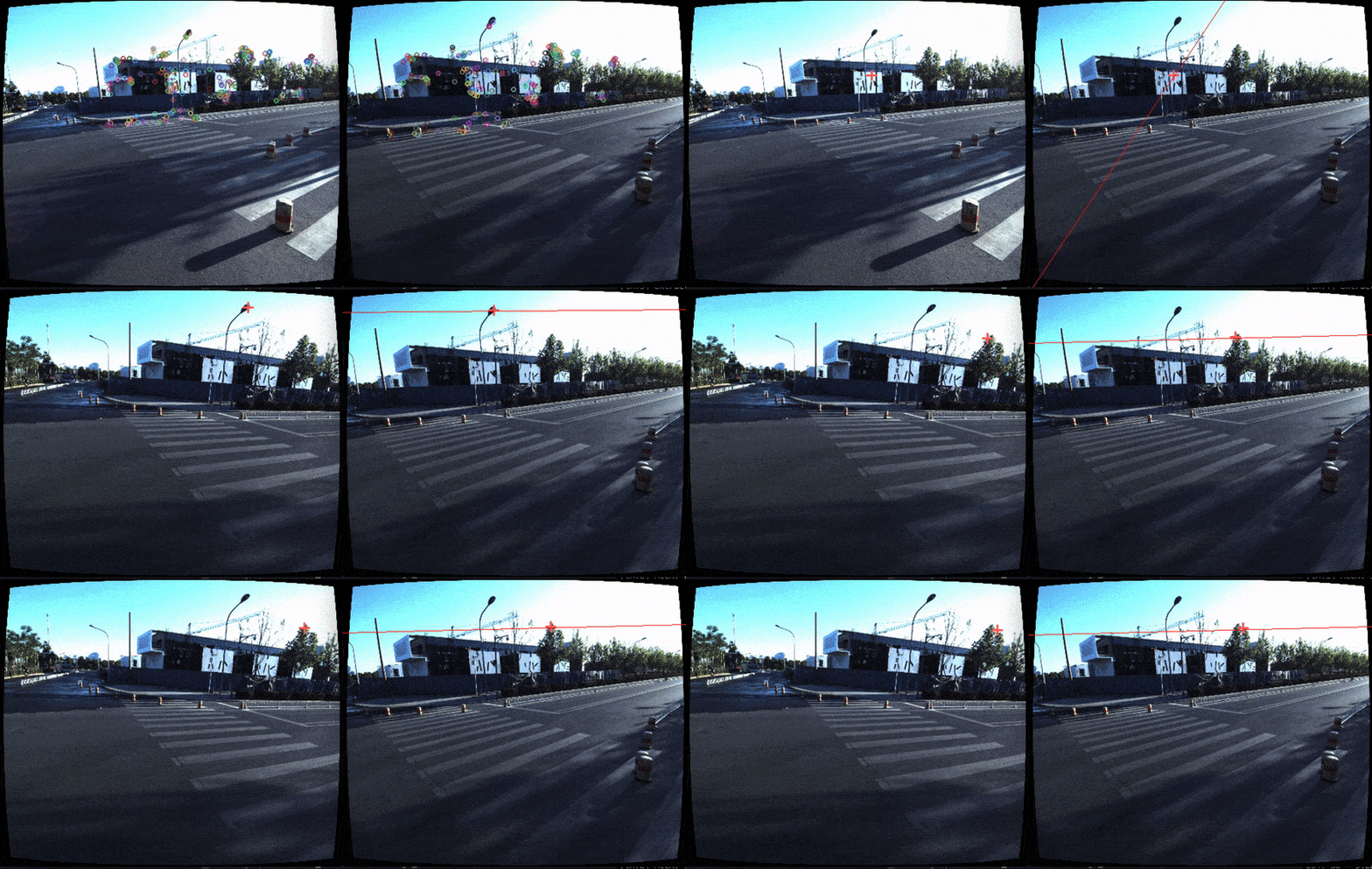
<p>An additional test for keypoint correspondence is the epipolar constraint, which can be applied by having camera poses and computed fundamental matrix between two cameras. So I checked the distance between keypoints and the correspondent epipolar line, and then filtered the keypoints with a distance larger than threshold values (default is <code class="language-plaintext highlighter-rouge">10px</code>).</p>

<div class="fig figcenter fighighlight">
  <img src="/imgs/apolloscape_sfm/line_constraints.gif" />
  <div class="margin:0">Epipolar constraint test and the visualization of points with a distance more than 10px from the epipolar line.</div>
</div>

<p>The last step is to filter image pairs that have the small number of matched keypoints remaining after Lowe’s ratio test and epipolar constraint filtering. I set the value to <code class="language-plaintext highlighter-rouge">seven</code> matched points for small reconstructions (up to <code class="language-plaintext highlighter-rouge">200</code> images) and approximately <code class="language-plaintext highlighter-rouge">60</code> points for reconstructions with more than <code class="language-plaintext highlighter-rouge">1000</code> images.</p>

<div class="fig figcenter fighighlight">
  <img src="/imgs/apolloscape_sfm/features_matched.png" />
  <div class=" margin:0">215 matched keypoints after all filter steps.</div>
</div>

<p>Another important consideration was how to make image pairs for keypoints matching. The easiest way is to generate all pairs, but it takes too long to match the features for all image combinations. We can instead reduce the number of pairs because we know camera locations and thus include only pairs with cameras that are located nearby.</p>

<p>After we extract keypoints from images and match image pairs, we create a connected components graph to quickly find images with the most common connections. Here is an example of building connected components for three images.</p>

<p>First, we have one image pair <code class="language-plaintext highlighter-rouge">[1,2]</code>:</p>

<div class="fig figcenter fighighlight">
  <img src="/imgs/apolloscape_sfm/match_1_2.png" />
  <div class=" margin:0">Connected components for one image pair [1,2].</div>
</div>

<p>Then we add image pair <code class="language-plaintext highlighter-rouge">[1,3]</code> and continue connecting keypoints into components:</p>

<div class="fig figcenter fighighlight">
  <img src="/imgs/apolloscape_sfm/match_1_2_3.png" />
  <div class=" margin:0">Connected components for two image pairs [1,2] and [1,3].</div>
</div>

<p>And finally we add matches for third image pair <code class="language-plaintext highlighter-rouge">[2,3]</code>:</p>

<div class="fig figcenter fighighlight">
  <img src="/imgs/apolloscape_sfm/match_1_2_3_all.png" />
  <div class=" margin:0">Connected components for three image pairs [1,2], [1,3] and [2,3].</div>
</div>

<p>Internally connected components are implemented as a tree, with the balanced depth of the subtrees, in order to support fast find and union operation. Fast check for connectedness is important in the merge-maps step, when we need to check whether points belong to the same component and therefore can be merged.</p>

<h2 id="initial-triangulation">Initial Triangulation</h2>

<p>The best image pair is the one with the most matched keypoints, so we can use it for the initial triangulation step. The more keypoints we have from the first image pair in the reconstruction, the greater the chance that we will have to connect corresponding 3D points from different image pairs in subsequent steps.</p>

<p>It’s also important to have connected points because Bundle Adjustment Optimization will tie different point clouds together and minimize re-projection errors from the same 3D point on multiple images.</p>

<div class="fig figcenter fighighlight">
  <img src="/imgs/apolloscape_sfm/best_match_rec8.png" />
  <div class=" margin:0">The best match during Record008 reconstruction. 1,089 keypoints matched.</div>
</div>

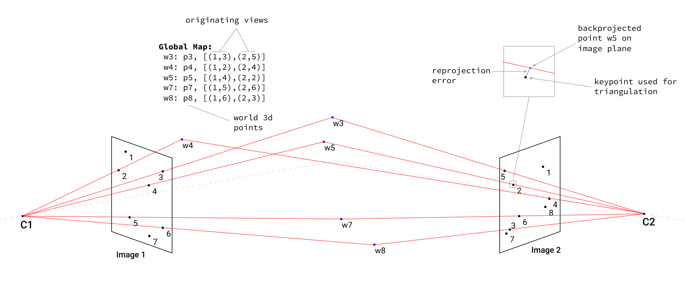
<p>Linear triangulation is implememnted using the classical DLT methods described in Hartley/Zisserman (12.2 p312) <a href="#references">[12]</a> which describes finding a solution for the system of equations <code class="language-plaintext highlighter-rouge">Ax=0</code> via SVD decomposition and taking the vector with the smallest singular value. For this purpose I used OpenCV function <code class="language-plaintext highlighter-rouge">cv::triangulatePoints</code> which is a pure SVD-based method.</p>

<p>For every 3D point, we are storing the list of both views and keypoints used to reconstruct this point.</p>

<div class="fig figcenter fighighlight">
  <img src="/imgs/apolloscape_sfm/recon_1_2_2x.png" />
  <div class=" margin:0">Example of initial image pair [1,2] triangulation.</div>
</div>

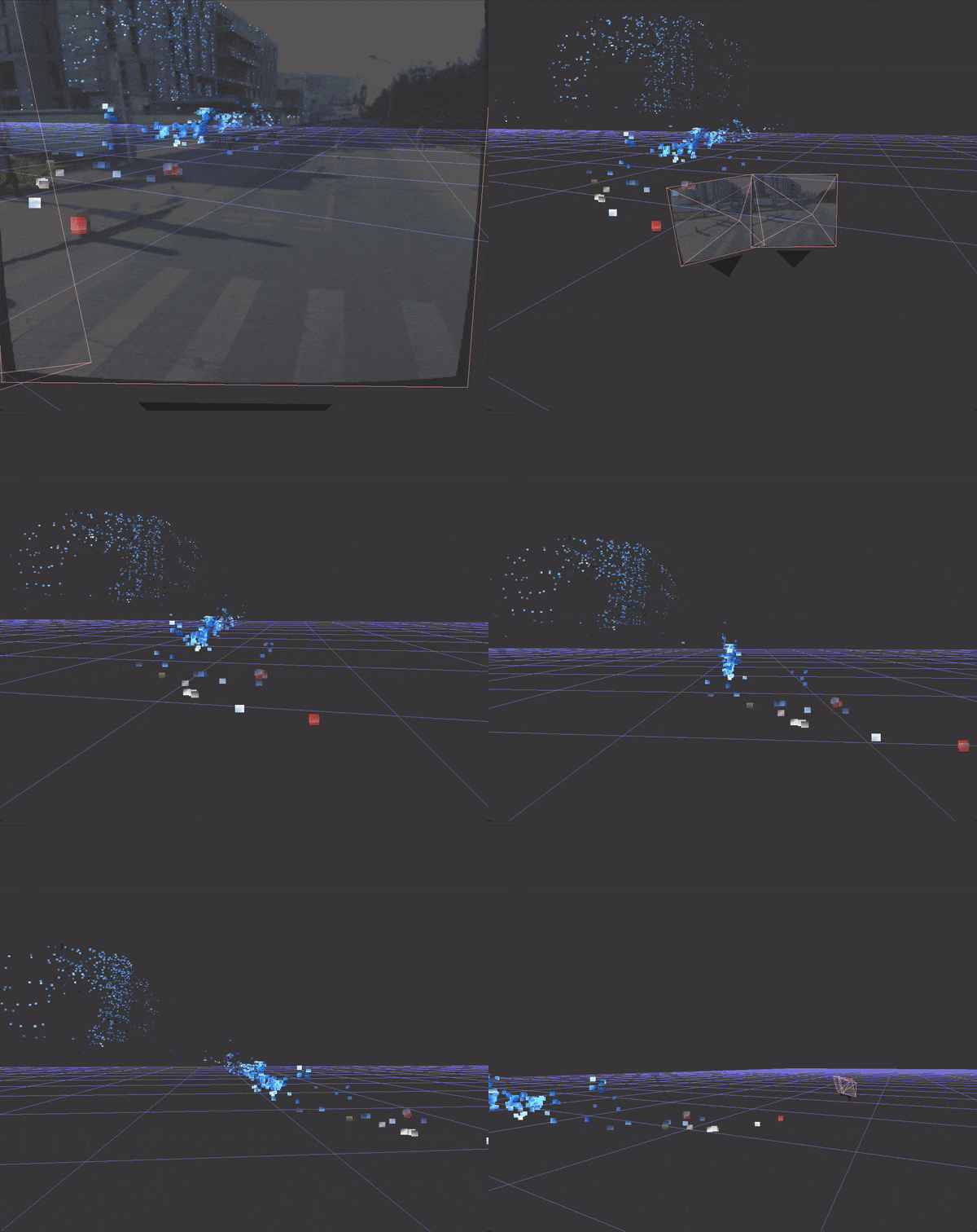
<p>Initial reconstruction step in 3D visualization, with filtered outliers and Bundle Adjustment Optimization that further minimizes the re-projection error of the survived points.</p>

<div class="fig figcenter fighighlight">
  <img src="/imgs/apolloscape_sfm/init_recon_opt.gif" />
  <div class=" margin:0">Initial reconstruction of the best match image pair for Record008.</div>
</div>

<h2 id="adding-of-other-images-and-merging-of-maps">Adding of Other Images and Merging of Maps</h2>

<p>We then check the most connected image from the list of unprocessed views against the list of the views that were already used for reconstruction. Next, we iterate the previous step until all views are used. Finally, we triangulate the corresponding pairs to obtain the local point cloud.</p>

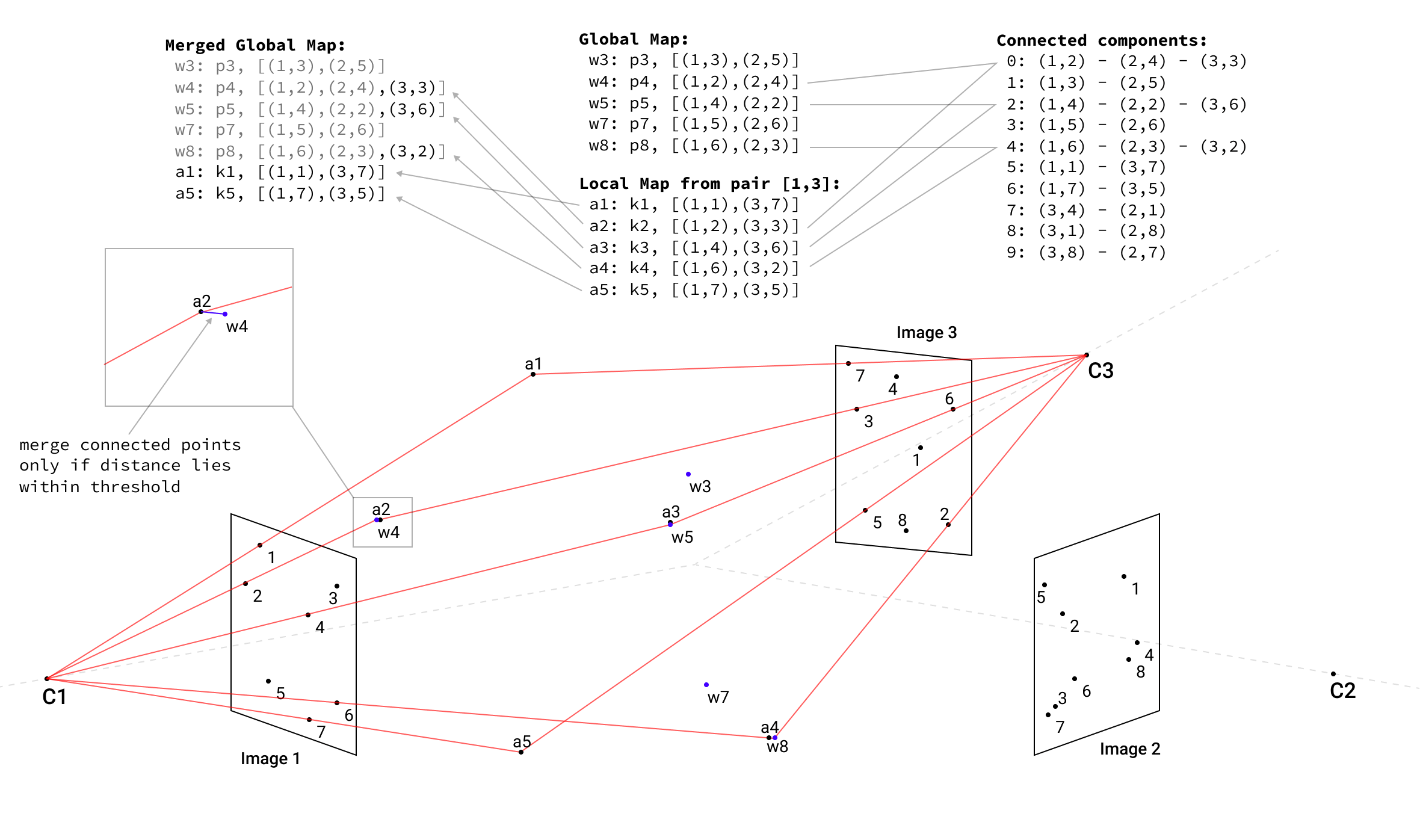
<p>Then local point clouds are merged into the global map along the points that belong to the same connected component, if the distance between two connected points lies within the threshold of <code class="language-plaintext highlighter-rouge">3.0m</code> (hyperparameter).</p>

<div class="fig figcenter fighighlight">
  <img src="/imgs/apolloscape_sfm/merge_map_2x_new.png" />
  <div class=" margin:0">Merged maps from the reconstruction of a subsequent view [1,3].</div>
</div>

<p>If the distance between connected points is bigger than the threshold, we discard both points from the map. Distinctive points without a connected points counterpart are copied to the global map without changes.</p>

<p>Below is an example of three subsequent steps after the initial reconstruction and its 3D visualization.</p>

<div class="fig figcenter fighighlight">
  <img src="/imgs/apolloscape_sfm/init_with3steps.png" />
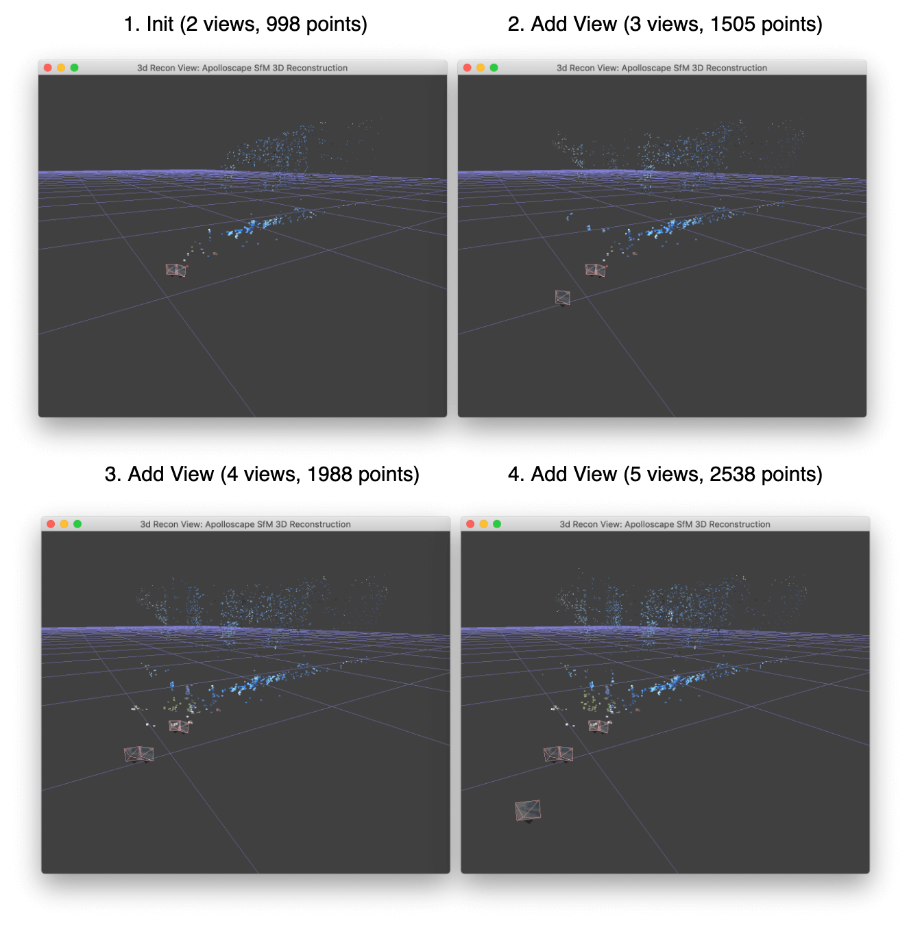
  <div class=" margin:0">Initial reconstruction and three next steps for Record008.</div>
</div>

<p>Thus we are increasing the resulting map with more and more 3D points while processing additional views.</p>

<h2 id="bundle-adjustment-optimization">Bundle Adjustment Optimization</h2>

<p>After every step of merging the map and increasing the views list of 3D points, we can perform map optimization and jointly minimize the re-projection error for every point on every originating view.</p>

<p>Mathematically, the problem statement is to minimize the loss function:</p>

\[\min_{\mathbf{\hat{X}_j}} \sum_{ij} d(P^i \mathbf{\hat{X}_j}, x_j^i)^2\]

<p>where \(d(a, b)\) is the geometric distance between two points; \(\mathbf{\hat{X}_j}\) is an estimated 3D point in a world space; \(P^i\) is a projection matrix for camera \(i\), \(x_j^i\) is 2D coordinates of a keypoint in image \(i\) that corresponds to the 3D point \(\mathbf{\hat{X}_j}\) and \(P^i \mathbf{\hat{X}_j}\) is a backprojection of point \(\mathbf{\hat{X}_j}\) to image \(i\).</p>

<p>I need to mention that this is a simpler formulation than usually encountered in full SLAM problems because we are not optimizing camera projection matrix \(P^i\) here (It’s known in the Apolloscape dataset). Furthermore, there is also no weighted matrix that accounts for variances in error contributions between different world points.</p>

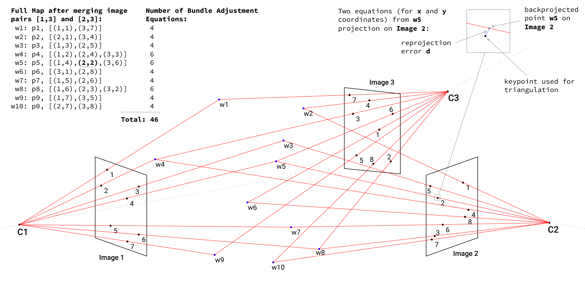
<p>Below, we continue the reconstruction of our three image examples with the resulting merged map of ten 3D points that correspond to <code class="language-plaintext highlighter-rouge">46</code> equations in the Bundle Adjustment Optimization problem.</p>

<div class="fig figcenter fighighlight">
  <img src="/imgs/apolloscape_sfm/bundle_adj_2x.png" />
  <div class=" margin:0">Bundle Adjustment Optimization for three image pairs.</div>
</div>

<p>Without camera poses computation, as in a full SLAM problem, we set only 3D map points as parameters to the Ceres solver, which performs Non-linear Least Squares optimization using the Levenberg-Marquardt method.</p>

<p>Ceres solver was optimized to work with huge problems, so the optimizations of <code class="language-plaintext highlighter-rouge">1.4M</code> 3D points is not too large for the library to handle (though it is demanding for CPU computation on my MacBook Pro:)</p>

<p>In order to save computation time, I run a Bundle Adjustment Optimization with Ceres solver only after I merge <code class="language-plaintext highlighter-rouge">40k</code> new 3D points to the global map. Such a sparse optimization approach works because the problem is a constraint in just 3D map-point optimization with known camera poses, and thus is more or less localized in the parameter space. There also no such events like loop closures, as in SLAM problems, which might wreak havoc on the map without a proper optimization of the current graph reconstruction.</p>

<h2 id="visualization">Visualization</h2>

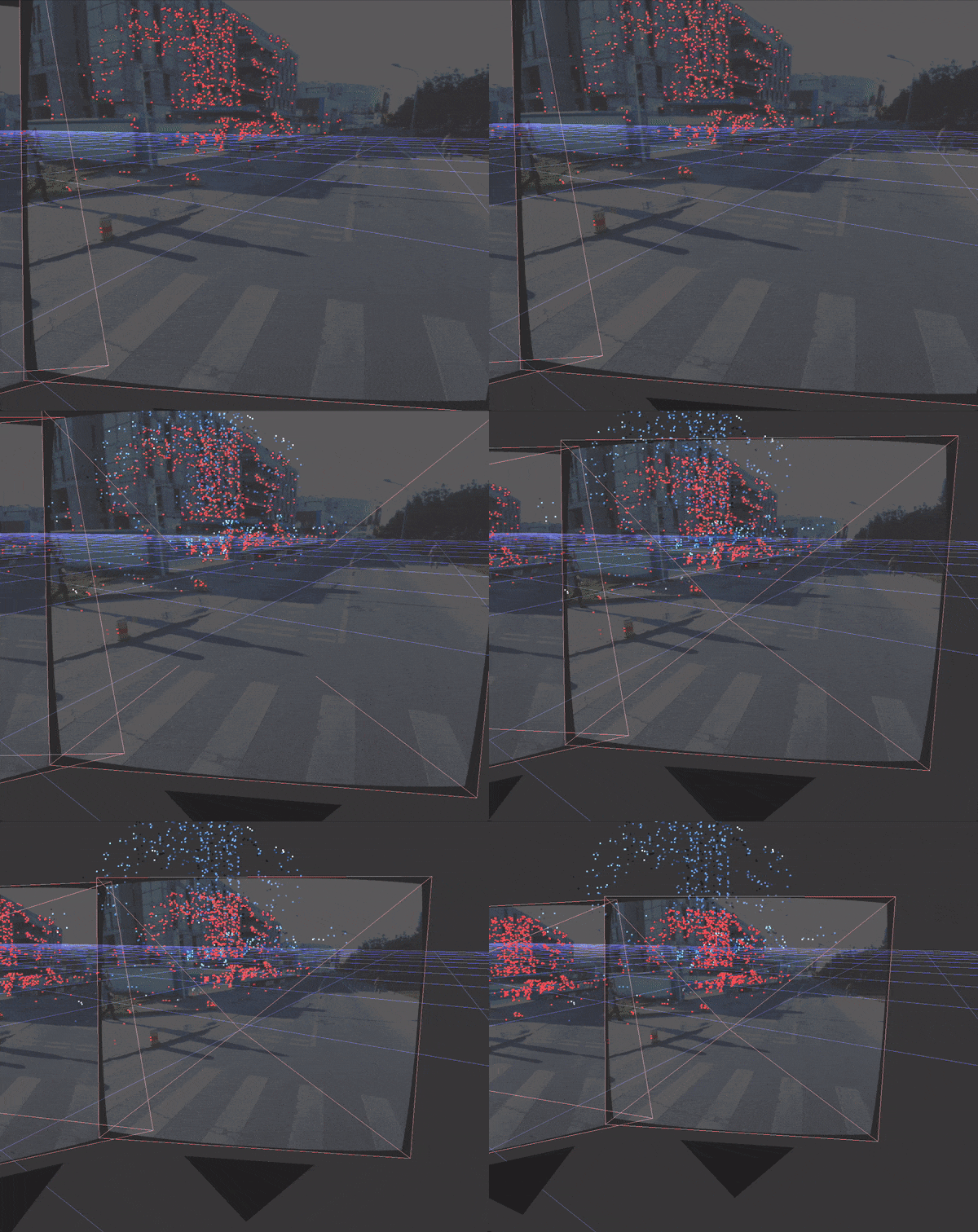
<p>I visualize the 3D map, cameras, images, and back-projection points with OpenGL using GLFW, glad, glm and OpenCV for key-points visualization. The idea behind is to have camera parameters for OpenGL visualization identical to camera parameters of the dataset; this provides more intuition in multi-view projective geometry to allow for the exploration of the scene reconstruction, camera projections, and locations in one environment.</p>

<div class="fig figcenter fighighlight">
  <img src="/imgs/apolloscape_sfm/points_alignment_backprojection.gif" />
  <div class=" margin:0">Camera alignment, with back-projection points, rendered on an image plane.</div>
</div>

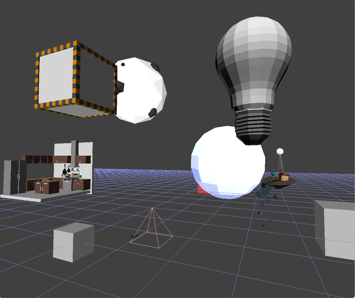
<p>Everything in visualization is done with vertices, vertex array buffers, vertex/fragment/geometry shaders, and ambient and diffuse lightning. In addition, the functionality to load arbitrary 3D objects from common file formats (.obj, .fbx via assimp library) is helpful as visual clues for some experiments.</p>

<div class="fig figcenter fighighlight">
  <img src="/imgs/apolloscape_sfm/3d_visual_env_crop.png" />
  <div class=" margin:0">Any 3D helper objects can be added to the environment.</div>
</div>

<p>As for 3D points visualization, we can add color information estimated from keypoint vertices. Every point represented as a square with four distinctive colors on the vertices as a texture. Vertex colors are estimated as the average colors extracted from pixels of the corresponding vertices for every connected keypoint, adjusted to the rotation angle and the size of the keypoints.</p>

<div class="fig figcenter fighighlight">
  <img src="/imgs/apolloscape_sfm/3d_squares.png" />
  <div class=" margin:0">Keypoints as squares with texture color information in the vertices (Four estimated color points).</div>
</div>

<p>This method provides a good understanding of keypoints and the region from which they were extracted (building, tree, road, etc.). However, many possible improvements can be done, for example, to add a center color point or to extract colors from the corresponding scaled version of the image. These methods allow for various keypoints octave and the visualization of squares in different sizes that account for variations in keypoint size.</p>

<h2 id="conclusion">Conclusion</h2>

<p>SfM is a classical pipeline that is still widely used in SLAM, Visual Odometry, and Localization approaches.</p>

<p>Having completed this project, I can now much better appreciate the challenges of common computer vision problems, their algorithmic and computational complexities, the difficulty of getting 3D space back from the 2D images, as well as the importance of visualization tools and intuition in understanding algorithms that form the basis of software in AR glasses, VR headsets, and self-driving robots.</p>

<p>While finishing this write up, I discovered the new Localization challenge for CVPR 2019 as part of the workshop <a href="https://sites.google.com/view/ltvl2019">“Long-Term Visual Localization under Changing Conditions”</a>. You can learn more at <a href="https://visuallocalization.net/">visuallocalization.net</a> <a href="#references">[16]</a></p>

<p>Yep, seems like I’ve found a new interesting problem and open datasets to play with for my next side project :)</p>

<p><a name="references"></a></p>

<h2 id="references">References</h2>

<ol>
  <li>Kendall, Alex, and Roberto Cipolla. <a href="https://arxiv.org/abs/1704.00390">“Geometric loss functions for camera pose regression with deep learning.”</a> (2017).</li>
  <li>Kendall, Alex, Matthew Grimes, and Roberto Cipolla. <a href="https://arxiv.org/abs/1505.07427">“Posenet: A convolutional network for real-time 6-dof camera relocalization.”</a> (2015).</li>
  <li>Schonberger, Johannes L., and Jan-Michael Frahm. <a href="https://www.cv-foundation.org/openaccess/content_cvpr_2016/papers/Schonberger_Structure-From-Motion_Revisited_CVPR_2016_paper.pdf">“Structure-from-motion revisited.”</a> (2016).</li>
  <li>COLMAP: general-purpose Structure-from-Motion (SfM) and Multi-View Stereo (MVS) pipeline with a graphical and command-line interface. <a href="https://colmap.github.io/">Project Page</a> (2016).</li>
  <li>MVE: an implementation of a complete end-to-end pipeline for image-based geometry reconstruction. <a href="https://www.gcc.tu-darmstadt.de/home/proj/mve/">Project Page</a></li>
  <li>openMVG: “open Multiple View Geometry” <a href="http://imagine.enpc.fr/~moulonp/openMVG/">Project Page</a></li>
  <li>VisualSFM : A Visual Structure from Motion System <a href="http://ccwu.me/vsfm/">Project Page</a></li>
  <li>Bundler: Structure from Motion (SfM) for Unordered Image Collections <a href="http://www.cs.cornell.edu/~snavely/bundler/">Project Page</a></li>
  <li>PMVS2: Patch-based Multi-view Stereo Software (PMVS - Version 2) <a href="https://www.di.ens.fr/pmvs/">PMVS2 Project Page</a> &amp; <a href="https://github.com/pmoulon/CMVS-PMVS">CMVS Project Page</a></li>
  <li>Tareen, Shaharyar Ahmed Khan, and Zahra Saleem. <a href="https://www.researchgate.net/publication/323561586_A_comparative_analysis_of_SIFT_SURF_KAZE_AKAZE_ORB_and_BRISK">“A comparative analysis of sift, surf, kaze, akaze, orb, and brisk.”</a> (2018).</li>
  <li>Lowe, David G. <a href="https://www.cs.ubc.ca/~lowe/papers/ijcv04.pdf">“Distinctive image features from scale-invariant keypoints.”</a> (2004).</li>
  <li>Hartley, Richard, and Andrew Zisserman. “Multiple view geometry in computer vision” (2003).</li>
  <li>Alcantarilla, Pablo F., and T. Solutions. <a href="http://www.bmva.org/bmvc/2013/Papers/paper0013/abstract0013.pdf">“Fast explicit diffusion for accelerated features in nonlinear scale spaces.”</a> (2011)</li>
  <li>Learn OpenGL - Modern OpenGL tutorial <a href="https://learnopengl.com/">https://learnopengl.com/</a></li>
  <li>Brahmbhatt, Samarth, et al. <a href="https://arxiv.org/abs/1712.03342">“Mapnet: Geometry-aware learning of maps for camera localization.”</a> (2017).</li>
  <li>Sattler, Torsten, et al. <a href="http://openaccess.thecvf.com/content_cvpr_2018/papers/Sattler_Benchmarking_6DOF_Outdoor_CVPR_2018_paper.pdf">“Benchmarking 6dof outdoor visual localization in changing conditions.”</a> (2018).</li>
</ol>]]></content><author><name>Pavlo Bashmakov</name></author><category term="blog" /><summary type="html"><![CDATA[Last year at CVPR 2018, I became interested in the Apolloscape dataset and the localization task challenge that was announced for ECCV 2018. I dived into the problem: exploring the Apolloscape dataset and using PoseNet with geometric loss functions [1,2] for direct pose prediction from monocular images. As a result, I got more interested in geometric approaches and multi-view geometry for computer vision tasks.]]></summary></entry><entry><title type="html">PoseNet implementation for self-driving car localization using Pytorch on Apolloscape dataset</title><link href="/blog/2018/08/24/apolloscape-posenet-pytorch.html" rel="alternate" type="text/html" title="PoseNet implementation for self-driving car localization using Pytorch on Apolloscape dataset" /><published>2018-08-24T08:00:00+00:00</published><updated>2018-08-24T08:00:00+00:00</updated><id>/blog/2018/08/24/apolloscape-posenet-pytorch</id><content type="html" xml:base="/blog/2018/08/24/apolloscape-posenet-pytorch.html"><![CDATA[<p>Localization is an essential task for augmented reality, robotics, and self-driving car applications. It’s crucial for a system to know the exact pose (location and orientation) of the agent to do visualization, navigation, prediction, and planning.</p>

<p>Baidu released its massive self-driving Apolloscape dataset in March and now has a couple of ongoing challenges for <a href="http://apolloscape.auto/ECCV/index.html">ECCV 2018 Workshop: Vision-based Navigation</a> for Autonomous Driving conference:</p>

<ul>
  <li>Task 1: Vision-based fine-grained lane markings segmentation</li>
  <li>Task 2: Self-localization on the fly</li>
  <li>Task 3: 3D car instance understanding</li>
</ul>

<p>I pick the self-localization problem and create the whole pipeline to localize a car which is based only on camera images.</p>

<p>This article covers the very beginning of the journey and includes the reading and visualization of the Apolloscape dataset for localization task. Implement PoseNet [<a href="#references">2</a>] architecture for monocular image pose prediction and visualize results. I use Python and Pytorch for the task.</p>

<p><strong><em>NOTE</em></strong>: If you want to jump straight to the code here is the <a href="https://github.com/bexcite/apolloscape-loc">GitHub repo</a>. It’s is still an ongoing work where I intend to implement Vidloc [<a href="#references">7</a>], Pose Graph Optimization [<a href="#references">3,8</a>] and Structure from Motion [<a href="#references">9</a>] pipelines for Apolloscape Dataset in the context of the localization task.</p>

<p><strong><em>NOTE 2</em></strong> (<em>update Mar 12, 2019</em>): Today I’m releasing the <a href="/blog/2019/03/12/apolloscape-sfm.html">second part of my journey</a> with Structure from Motion (SfM) pipeline and OpenGL visualization for Apolloscape ZPark Sample implemented on C++.</p>

<h2 id="apolloscape-dataset">Apolloscape Dataset</h2>

<p>Apolloscape dataset emerged from the Baidu effort in 2017 to collect enough data with the modern sensors that can be used for self-driving car research. Dataset provides camera images, poses, dense LIDAR point clouds, 3d semantic maps, 3d lane markings, 2d segmentation labels. Eventually, they plan to reach 200K images, captured on 20km roads covering 5 sites from 3 cities. Initial dataset was released in March 2018 and continuously updated for the ongoing ECCV challenges.</p>

<p>For the challenge purpose, Apolloscape provides separate archives for the self-localization task. You can download the small (4Gb) <code class="language-plaintext highlighter-rouge">self-localization-examples</code> ZPark from <a href="http://apolloscape.auto/self_localization.html#to_dataset_href">Self-Localization Dataset</a> page.</p>

<p>I use ZPark sample dataset for almost everything in this article from visualization to PoseNet training.</p>

<h2 id="apolloscape-pytorch-dataset">Apolloscape Pytorch Dataset</h2>

<p>For Pytorch I need to have a <code class="language-plaintext highlighter-rouge">Dataset</code> object that prepares and feeds the data to the loader and then to the model. I want to have a robust dataset class that can:</p>
<ul>
  <li>support stereo and mono images</li>
  <li>support train/validation splits that came along with data or generate a new one</li>
  <li>support pose normalization</li>
  <li>support different pose representations (needed mainly for visualization and experiments with loss functions)</li>
  <li>support filtering by record id</li>
  <li>support general Apolloscape folder structure layout</li>
</ul>

<p>I am not putting here the full listing of the <code class="language-plaintext highlighter-rouge">Apolloscape</code> dataset and concentrate solely on how to use it and what data we can get from it. For the full source code, please refer to the Github file <a href="https://github.com/bexcite/apolloscape-loc/blob/master/datasets/apolloscape.py"><code class="language-plaintext highlighter-rouge">datasets/apolloscape.py</code></a>.</p>

<p>Here how to create a dataset:</p>

<div class="language-python highlighter-rouge"><div class="highlight"><pre class="highlight"><code><span class="kn">from</span> <span class="nn">datasets.apolloscape</span> <span class="kn">import</span> <span class="n">Apolloscape</span>
<span class="kn">from</span> <span class="nn">torchvision</span> <span class="kn">import</span> <span class="n">transforms</span>

<span class="c1"># Path to unpacked data folders
</span><span class="n">APOLLO_PATH</span> <span class="o">=</span> <span class="s">"./data/apolloscape"</span>

<span class="c1"># Resize transform that is applied on every image read
</span><span class="n">transform</span> <span class="o">=</span> <span class="n">transforms</span><span class="p">.</span><span class="n">Compose</span><span class="p">([</span><span class="n">transforms</span><span class="p">.</span><span class="n">Resize</span><span class="p">(</span><span class="mi">250</span><span class="p">)])</span>

<span class="n">apollo_dataset</span> <span class="o">=</span> <span class="n">Apolloscape</span><span class="p">(</span><span class="n">root</span><span class="o">=</span><span class="n">os</span><span class="p">.</span><span class="n">path</span><span class="p">.</span><span class="n">join</span><span class="p">(</span><span class="n">APOLLO_PATH</span><span class="p">),</span> <span class="n">road</span><span class="o">=</span><span class="s">"zpark-sample"</span><span class="p">,</span>
                             <span class="n">transform</span><span class="o">=</span><span class="n">transform</span><span class="p">,</span> <span class="n">train</span><span class="o">=</span><span class="bp">True</span><span class="p">,</span> <span class="n">pose_format</span><span class="o">=</span><span class="s">'quat'</span><span class="p">,</span>
                             <span class="n">stereo</span><span class="o">=</span><span class="bp">True</span><span class="p">)</span>
<span class="k">print</span><span class="p">(</span><span class="n">apollo_dataset</span><span class="p">)</span>
</code></pre></div></div>

<p>Output:</p>
<pre><code class="language-Shell">Dataset: Apolloscape
    Road: zpark-sample
    Record: None
    Train: None
    Normalize Poses: False
    Stereo: True
    Length: 1499 of 1499
    Cameras: ['Camera_2', 'Camera_1']
    Records: ['Record001', 'Record002', 'Record003', 'Record004', 'Record006', 'Record007', 'Record008', 'Record009', 'Record010', 'Record011', 'Record012', 'Record013', 'Record014']
</code></pre>

<p><code class="language-plaintext highlighter-rouge">APOLLO_PATH</code> is a folder with unpacked Apolloscape datasets, e.g. <code class="language-plaintext highlighter-rouge">$APOLLO_PATH/road02_seg</code> or <code class="language-plaintext highlighter-rouge">$APOLLO_PATH/zpark</code>. Download data from Apolloscape page and unpack iot. Let’s assume that we’ve also created a symlink <code class="language-plaintext highlighter-rouge">./data/apolloscape</code> that points to <code class="language-plaintext highlighter-rouge">$APOLLO_PATH</code> folder.</p>

<p>We can view the list of available records with a number of data samples in each:</p>

<div class="language-python highlighter-rouge"><div class="highlight"><pre class="highlight"><code><span class="c1"># Show records with numbers of data points
</span><span class="n">recs_num</span> <span class="o">=</span> <span class="n">apollo_dataset</span><span class="p">.</span><span class="n">get_records_counts</span><span class="p">()</span>
<span class="n">recs_num</span> <span class="o">=</span> <span class="nb">sorted</span><span class="p">(</span><span class="n">recs_num</span><span class="p">.</span><span class="n">items</span><span class="p">(),</span> <span class="n">key</span><span class="o">=</span><span class="k">lambda</span> <span class="n">kv</span><span class="p">:</span> <span class="n">kv</span><span class="p">[</span><span class="mi">1</span><span class="p">],</span> <span class="n">reverse</span><span class="o">=</span><span class="bp">True</span><span class="p">)</span>
<span class="k">print</span><span class="p">(</span><span class="s">"Records:"</span><span class="p">)</span>
<span class="k">print</span><span class="p">(</span><span class="s">"</span><span class="se">\n</span><span class="s">"</span><span class="p">.</span><span class="n">join</span><span class="p">([</span><span class="s">"</span><span class="se">\t</span><span class="s">{} - {}"</span><span class="p">.</span><span class="nb">format</span><span class="p">(</span><span class="n">r</span><span class="p">[</span><span class="mi">0</span><span class="p">],</span> <span class="n">r</span><span class="p">[</span><span class="mi">1</span><span class="p">])</span> <span class="k">for</span> <span class="n">r</span> <span class="ow">in</span> <span class="n">recs_num</span> <span class="p">]))</span>
</code></pre></div></div>

<p>Output:</p>
<pre><code class="language-Shell">Records:
	Record008 - 122
	Record007 - 121
	Record006 - 121
	Record012 - 121
	Record001 - 121
	Record009 - 121
	Record010 - 121
	Record003 - 121
	Record013 - 120
	Record004 - 120
	Record002 - 120
	Record011 - 120
	Record014 - 50
</code></pre>

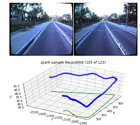
<p>We can draw a route for one record with a sampled camera image:</p>
<div class="language-python highlighter-rouge"><div class="highlight"><pre class="highlight"><code><span class="kn">from</span> <span class="nn">utils.common</span> <span class="kn">import</span> <span class="n">draw_record</span>

<span class="c1"># Draw path of a record with a sampled datapoint
</span><span class="n">record</span> <span class="o">=</span> <span class="s">'Record008'</span>
<span class="n">draw_record</span><span class="p">(</span><span class="n">apollo_dataset</span><span class="p">,</span> <span class="n">record</span><span class="p">)</span>
<span class="n">plt</span><span class="p">.</span><span class="n">show</span><span class="p">()</span>
</code></pre></div></div>

<p>Output:</p>

<div class="fig figcenter fighighlight">
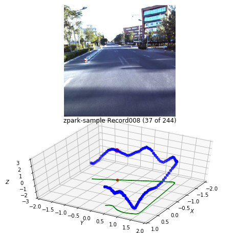
  <img src="/imgs/apolloscape_posenet/draw_record_008.png" />
  <div class="figcaption figcenter">Record008 path and sampled stereo images pair (top). Blue - record path. Red  - image pair location. Green - path projection on z-plane.</div>
</div>

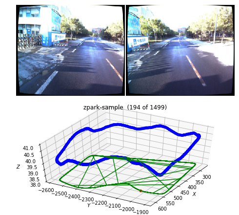
<p>Alternatively, we can see all records at once in one chart:</p>
<div class="language-python highlighter-rouge"><div class="highlight"><pre class="highlight"><code><span class="c1"># Draw all records for current dataset
</span><span class="n">draw_record</span><span class="p">(</span><span class="n">apollo_dataset</span><span class="p">)</span>
<span class="n">plt</span><span class="p">.</span><span class="n">show</span><span class="p">()</span>
</code></pre></div></div>

<p>Output:</p>

<div class="fig figcenter fighighlight">
  <img src="/imgs/apolloscape_posenet/draw_record_all.png" />
  <div class="figcaption figcenter">All records from the dataset on one chart. Path projection connects the end of one record and the beginning of the next record.</div>
</div>

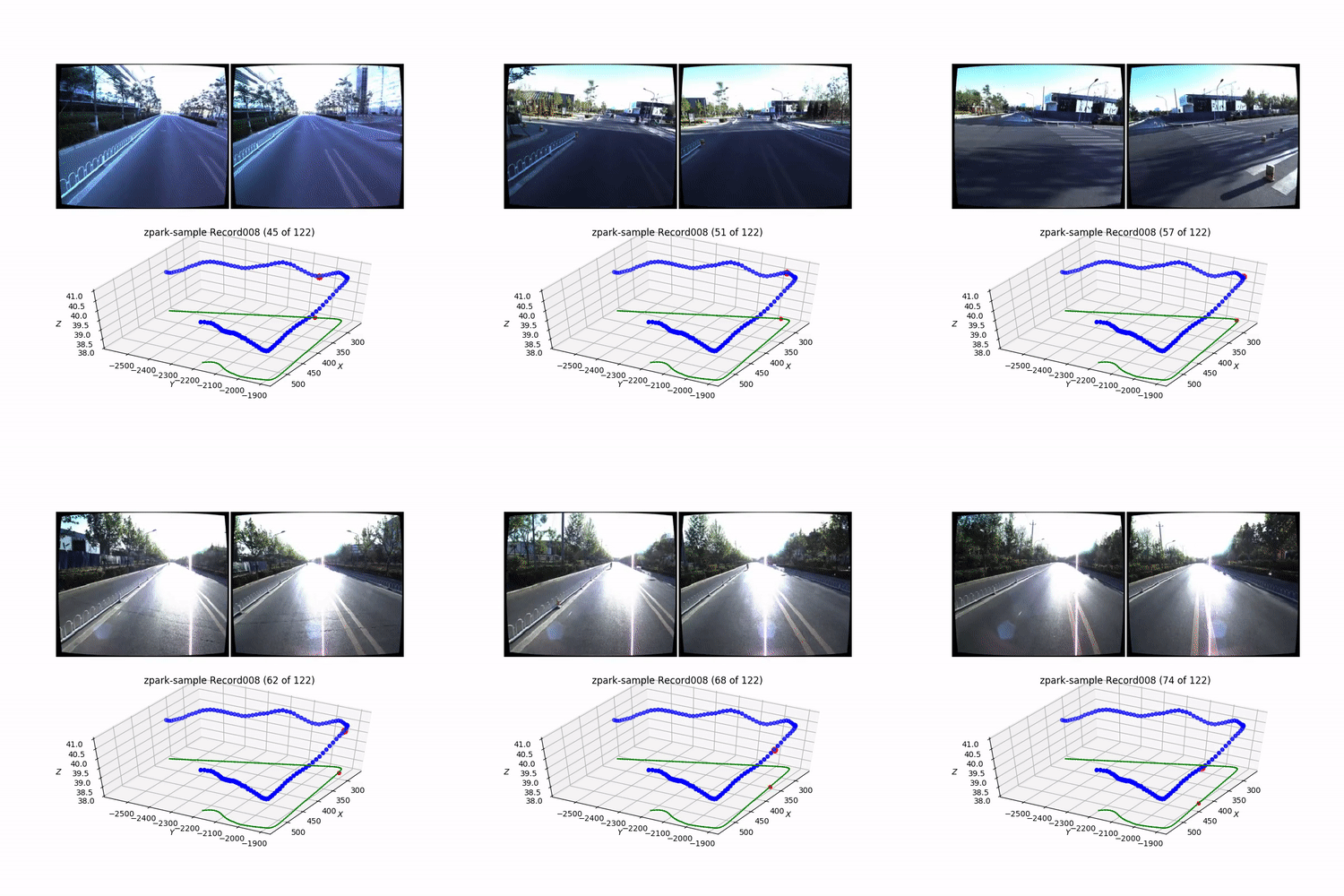
<p>Another option is to see it in a video:</p>
<div class="language-python highlighter-rouge"><div class="highlight"><pre class="highlight"><code><span class="kn">from</span> <span class="nn">utils.common</span> <span class="kn">import</span> <span class="n">make_video</span>

<span class="c1"># Generate and save video for the record
</span><span class="n">outfile</span> <span class="o">=</span> <span class="s">"./output_data/videos/video_{}_{}.mp4"</span><span class="p">.</span><span class="nb">format</span><span class="p">(</span><span class="n">apollo_dataset</span><span class="p">.</span><span class="n">road</span><span class="p">,</span> <span class="n">apollo_dataset</span><span class="p">.</span><span class="n">record</span><span class="p">)</span>
<span class="n">make_video</span><span class="p">(</span><span class="n">apollo_dataset</span><span class="p">,</span> <span class="n">outfile</span><span class="o">=</span><span class="n">outfile</span><span class="p">)</span>
</code></pre></div></div>

<p>Output (cut gif version of the generated video):</p>
<div class="fig figcenter fighighlight">
  <img src="/imgs/apolloscape_posenet/video_record_008_500.gif" />
  <div class="margin:0">Generated video sample for Record008</div>
</div>

<p>For the PoseNet training we will use mono images with zero-mean normalized poses and camera images center-cropped to 250px:</p>
<div class="language-python highlighter-rouge"><div class="highlight"><pre class="highlight"><code><span class="c1"># Resize and CenterCrop
</span><span class="n">transform</span> <span class="o">=</span> <span class="n">transforms</span><span class="p">.</span><span class="n">Compose</span><span class="p">([</span>
    <span class="n">transforms</span><span class="p">.</span><span class="n">Resize</span><span class="p">(</span><span class="mi">260</span><span class="p">),</span>
    <span class="n">transforms</span><span class="p">.</span><span class="n">CenterCrop</span><span class="p">(</span><span class="mi">250</span><span class="p">)</span>
<span class="p">])</span>

<span class="c1"># Create train dataset with mono images, normalized poses, enabled cache_transform
</span><span class="n">train_dataset</span> <span class="o">=</span> <span class="n">Apolloscape</span><span class="p">(</span><span class="n">root</span><span class="o">=</span><span class="n">os</span><span class="p">.</span><span class="n">path</span><span class="p">.</span><span class="n">join</span><span class="p">(</span><span class="n">APOLLO_PATH</span><span class="p">),</span> <span class="n">road</span><span class="o">=</span><span class="s">"zpark-sample"</span><span class="p">,</span>
                             <span class="n">transform</span><span class="o">=</span><span class="n">transform</span><span class="p">,</span> <span class="n">train</span><span class="o">=</span><span class="bp">True</span><span class="p">,</span> <span class="n">pose_format</span><span class="o">=</span><span class="s">'quat'</span><span class="p">,</span>
                             <span class="n">normalize_poses</span><span class="o">=</span><span class="bp">True</span><span class="p">,</span> <span class="n">cache_transform</span><span class="o">=</span><span class="bp">True</span><span class="p">,</span>
                             <span class="n">stereo</span><span class="o">=</span><span class="bp">False</span><span class="p">)</span>

<span class="c1"># Draw path of a single record (mono with normalized poses)
</span><span class="n">record</span> <span class="o">=</span> <span class="s">'Record008'</span>
<span class="n">draw_record</span><span class="p">(</span><span class="n">apollo_dataset</span><span class="p">,</span> <span class="n">record</span><span class="p">)</span>
<span class="n">plt</span><span class="p">.</span><span class="n">show</span><span class="p">()</span>
</code></pre></div></div>

<p>Output:</p>

<div class="fig figcenter fighighlight">
  <img src="/imgs/apolloscape_posenet/draw_record_008_mono_norm.png" />
  <div class="figcaption figcenter">Normalised poses and mono images resized and cropped to 250px.</div>
</div>

<p>Implemented Apolloscape Pytorch dataset also supports <code class="language-plaintext highlighter-rouge">cache_transform</code> option which is when enabled saves all transformed pickled images to a disk and retrieves it later for the subsequent epochs without the need to redo convert and transform operations every image read event. Cache saves up to 50% of the time during training time though it’s not working with image augmentation transforms like <code class="language-plaintext highlighter-rouge">torchvision.transforms.ColorJitter</code>.</p>

<p>Also, we can get the mean and the standard deviation that we need later to recover true poses translations:</p>

<div class="language-python highlighter-rouge"><div class="highlight"><pre class="highlight"><code><span class="n">poses_mean</span> <span class="o">=</span> <span class="n">train_dataset</span><span class="p">.</span><span class="n">poses_mean</span>
<span class="n">poses_std</span> <span class="o">=</span> <span class="n">train_dataset</span><span class="p">.</span><span class="n">poses_std</span>
<span class="k">print</span><span class="p">(</span><span class="s">'Translation poses_mean = {} in meters'</span><span class="p">.</span><span class="nb">format</span><span class="p">(</span><span class="n">poses_mean</span><span class="p">))</span>
<span class="k">print</span><span class="p">(</span><span class="s">'Translation poses_std  = {} in meters'</span><span class="p">.</span><span class="nb">format</span><span class="p">(</span><span class="n">poses_std</span><span class="p">))</span>
</code></pre></div></div>

<p>Output:</p>
<pre><code class="language-Shell">Translation poses_mean = [  449.95782055 -2251.24771214    40.17147932] in meters
Translation poses_std  = [123.39589457 252.42350964   0.28021513] in meters
</code></pre>

<p>You can find all mentioned examples in <a href="https://github.com/bexcite/apolloscape-loc/blob/master/Apolloscape_View_Records.ipynb"><code class="language-plaintext highlighter-rouge">Apolloscape_View_Records.ipynb</code></a> notebook.</p>

<p>And now let’s turn to something useful and more interesting, for example, training PoseNet deep convolutional network to regress poses from camera images.</p>

<h1 id="posenet-localization-task">PoseNet localization task</h1>

<p>In general case, online localization task formulation goes like this: find the current robot pose \(\mathbf{X}_t\) given its previous state \(\mathbf{X}_{t-1}\) and current sensors observations \(\mathbf{Z}_t\):</p>

\[\mathbf{X}_t = f( \mathbf{X}_{t-1}, \mathbf{Z}_{t} )\]

<p>PoseNet deep convolutional neural network regresses robot pose from monocular image; thus we are not taking in account previous robot state \(\mathbf{X}_{t-1}\) at all:</p>

\[\mathbf{X}_t = f( \mathbf{Z}_t )\]

<p>Our observation sensor is a camera that gives us a monocular image \(\mathbf{I}_t\). After removing subscript indexes for simplicity, we can define our task as to find a pose \(\mathbf{X}\) given a monocular image \(\mathbf{I}\).</p>

\[\mathbf{X} = f( \mathbf{I} )\]

<p>where \(\mathbf{X}\) represents the full pose with translation \(\mathbf{x}\) and rotation \(\mathbf{q}\) components:</p>

\[\mathbf{X} = [ \mathbf{x}, \mathbf{q} ] \\
\mathbf{x} = [x, y, z], \quad
\mathbf{q} = [ q_1, q_2, q_3, q_4]\]

<p>Rotation is represented in quaternions because they do not suffer from a wrap around \(2\pi\) radians as Euler angles or axis-angle representations and more straightforward to deal than 3x3 rotation matrices.</p>

<p>For more information about the selection of different pose representation for deep learning refer to the excellent paper <a href="https://arxiv.org/abs/1704.00390">“Geometric loss functions for camera pose regression with deep learning”</a> by Alex Kendall et al.</p>

<h2 id="posenet-architecture">PoseNet Architecture</h2>

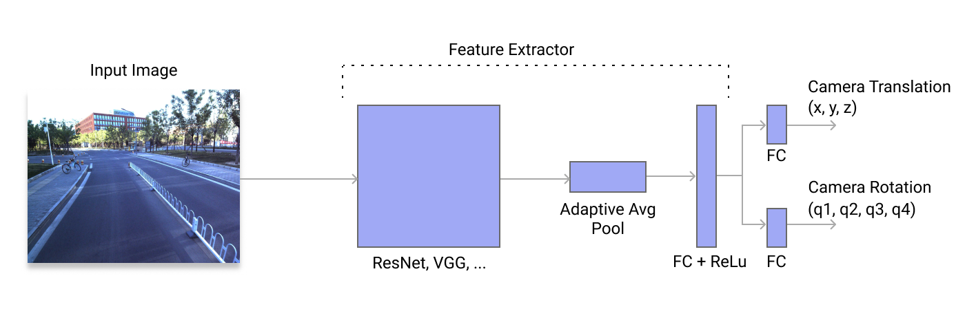
<p>I build a DNN-based regressor for camera pose on ResNet and modify it by adding a global average pooling layer after the last convolutional layer and introducing a fully-connected layer with 2048 neurons. Finally, it’s concluded with 6 DoF camera pose regressor for translation \((x, y, z)\), and rotation \((q_1, q_2, q_3, q_4)\) vectors.</p>

<div class="fig figcenter fighighlight">
  <img src="/imgs/apolloscape_posenet/posenet_arch.png" />
  <div class="figcaption figcenter">A PoseNet architecture with feature extractor network and regressors for camera translation and rotation. Feature extractor can be a pretrained on ImageNet ResNet18, ResNet34 or ResNet50.</div>
</div>

<p>A Pytorch implementation of the PoseNet model using a mono image:</p>

<div class="language-python highlighter-rouge"><div class="highlight"><pre class="highlight"><code><span class="kn">import</span> <span class="nn">torch</span>
<span class="kn">import</span> <span class="nn">torch.nn.functional</span> <span class="k">as</span> <span class="n">F</span>

<span class="k">class</span> <span class="nc">PoseNet</span><span class="p">(</span><span class="n">torch</span><span class="p">.</span><span class="n">nn</span><span class="p">.</span><span class="n">Module</span><span class="p">):</span>

    <span class="k">def</span> <span class="nf">__init__</span><span class="p">(</span><span class="bp">self</span><span class="p">,</span> <span class="n">feature_extractor</span><span class="p">,</span> <span class="n">num_features</span><span class="o">=</span><span class="mi">128</span><span class="p">,</span> <span class="n">dropout</span><span class="o">=</span><span class="mf">0.5</span><span class="p">,</span>
                 <span class="n">track_running_stats</span><span class="o">=</span><span class="bp">False</span><span class="p">,</span> <span class="n">pretrained</span><span class="o">=</span><span class="bp">False</span><span class="p">):</span>
        <span class="nb">super</span><span class="p">(</span><span class="n">PoseNet</span><span class="p">,</span> <span class="bp">self</span><span class="p">).</span><span class="n">__init__</span><span class="p">()</span>
        <span class="bp">self</span><span class="p">.</span><span class="n">dropout</span> <span class="o">=</span> <span class="n">dropout</span>
        <span class="bp">self</span><span class="p">.</span><span class="n">feature_extractor</span> <span class="o">=</span> <span class="n">feature_extractor</span>
        <span class="bp">self</span><span class="p">.</span><span class="n">feature_extractor</span><span class="p">.</span><span class="n">avgpool</span> <span class="o">=</span> <span class="n">torch</span><span class="p">.</span><span class="n">nn</span><span class="p">.</span><span class="n">AdaptiveAvgPool2d</span><span class="p">(</span><span class="mi">1</span><span class="p">)</span>
        <span class="n">fc_in_features</span> <span class="o">=</span> <span class="bp">self</span><span class="p">.</span><span class="n">feature_extractor</span><span class="p">.</span><span class="n">fc</span><span class="p">.</span><span class="n">in_features</span>
        <span class="bp">self</span><span class="p">.</span><span class="n">feature_extractor</span><span class="p">.</span><span class="n">fc</span> <span class="o">=</span> <span class="n">torch</span><span class="p">.</span><span class="n">nn</span><span class="p">.</span><span class="n">Linear</span><span class="p">(</span><span class="n">fc_in_features</span><span class="p">,</span> <span class="n">num_features</span><span class="p">)</span>

        <span class="c1"># Translation
</span>        <span class="bp">self</span><span class="p">.</span><span class="n">fc_xyz</span> <span class="o">=</span> <span class="n">torch</span><span class="p">.</span><span class="n">nn</span><span class="p">.</span><span class="n">Linear</span><span class="p">(</span><span class="n">num_features</span><span class="p">,</span> <span class="mi">3</span><span class="p">)</span>

        <span class="c1"># Rotation in quaternions
</span>        <span class="bp">self</span><span class="p">.</span><span class="n">fc_quat</span> <span class="o">=</span> <span class="n">torch</span><span class="p">.</span><span class="n">nn</span><span class="p">.</span><span class="n">Linear</span><span class="p">(</span><span class="n">num_features</span><span class="p">,</span> <span class="mi">4</span><span class="p">)</span>

    <span class="k">def</span> <span class="nf">extract_features</span><span class="p">(</span><span class="bp">self</span><span class="p">,</span> <span class="n">x</span><span class="p">):</span>
        <span class="n">x_features</span> <span class="o">=</span> <span class="bp">self</span><span class="p">.</span><span class="n">feature_extractor</span><span class="p">(</span><span class="n">x</span><span class="p">)</span>
        <span class="n">x_features</span> <span class="o">=</span> <span class="n">F</span><span class="p">.</span><span class="n">relu</span><span class="p">(</span><span class="n">x_features</span><span class="p">)</span>
        <span class="k">if</span> <span class="bp">self</span><span class="p">.</span><span class="n">dropout</span> <span class="o">&gt;</span> <span class="mi">0</span><span class="p">:</span>
            <span class="n">x_features</span> <span class="o">=</span> <span class="n">F</span><span class="p">.</span><span class="n">dropout</span><span class="p">(</span><span class="n">x_features</span><span class="p">,</span> <span class="n">p</span><span class="o">=</span><span class="bp">self</span><span class="p">.</span><span class="n">dropout</span><span class="p">,</span> <span class="n">training</span><span class="o">=</span><span class="bp">self</span><span class="p">.</span><span class="n">training</span><span class="p">)</span>
        <span class="k">return</span> <span class="n">x_features</span>

    <span class="k">def</span> <span class="nf">forward</span><span class="p">(</span><span class="bp">self</span><span class="p">,</span> <span class="n">x</span><span class="p">):</span>
        <span class="n">x_features</span> <span class="o">=</span> <span class="bp">self</span><span class="p">.</span><span class="n">extract_features</span><span class="p">(</span><span class="n">x</span><span class="p">)</span>
        <span class="n">x_translations</span> <span class="o">=</span> <span class="bp">self</span><span class="p">.</span><span class="n">fc_xyz</span><span class="p">(</span><span class="n">x_features</span><span class="p">)</span>
        <span class="n">x_rotations</span> <span class="o">=</span> <span class="bp">self</span><span class="p">.</span><span class="n">fc_quat</span><span class="p">(</span><span class="n">x_features</span><span class="p">)</span>
        <span class="n">x_poses</span> <span class="o">=</span> <span class="n">torch</span><span class="p">.</span><span class="n">cat</span><span class="p">((</span><span class="n">x_translations</span><span class="p">,</span> <span class="n">x_rotations</span><span class="p">),</span> <span class="n">dim</span><span class="o">=</span><span class="mi">1</span><span class="p">)</span>
        <span class="k">return</span> <span class="n">x_poses</span>
</code></pre></div></div>

<p>For further experiments I’ve also implemented stereo version (currently it’s simply processes two images in parallel without any additional constraints), option to switch off stats tracking for BatchNorm layers and Kaiming He normal for weight initialization [<a href="#references">4</a>]. Full source code is here <a href="https://github.com/bexcite/apolloscape-loc/blob/master/models/posenet.py"><code class="language-plaintext highlighter-rouge">models/posenet.py</code></a></p>

<h2 id="posenet-loss-functions">PoseNet Loss Functions</h2>

<p>As a loss function I use a weighted combination of losses for translation and orientation as described in the original PoseNet paper [<a href="#references">2</a>]:</p>

\[\mathcal{L}_{\beta} (\mathbf{I}) = \mathcal{L}_{x}(\mathbf{I}) + \beta \mathcal{L}_{q}(\mathbf{I})\]

<p>Scaling factor \(\beta\) was introduced to balance the losses of two variables expressed in different units and of different scales. Weighting param depends on the task itself and should be selected as a model hyper-parameter.</p>

<div class="fig figcenter fighighlight">
  <img src="/imgs/apolloscape_posenet/beta_graph.png" />
  <div class="figcaption figcenter">Example of parameter \( \beta \) influence on convnet performance on Chess scene from 7Scenes. <br />Source: Alex Kendall <a href="#references">[2]</a></div>
</div>

<p>The second option for a loss function is to use a learning approach to find an optimal weighting for translation and orientation:</p>

\[\mathcal{L}_{\sigma}(\mathbf{I}) = \frac{\mathcal{L}_x(\mathbf{I})}{\hat{\sigma}_x^2} +
\log \hat{\sigma}_x^2 + \frac{\mathcal{L}_q(\mathbf{I})}{\hat{\sigma}_q^2} +
\log \hat{\sigma}_q^2\]

<p>\( \hat{\sigma}_x^2, \hat{\sigma}_q^2 \), homoscedastic uncertainties, represent free scalar values that we learn through backpropagation with respect to the loss function. Their effect is to decrease or increase the corresponding loss component automatically. And \( \log \hat{\sigma}_x^2, \log \hat{\sigma}_q^2 \) are the corresponding regularizers that prevent these values to become too big.</p>

<p>In practice, to prevent the potential division by zero, authors [<a href="#references">1</a>] suggest learning \( \hat{s} := \log \hat{\sigma}^2 \) which is more numerically stable. So the final loss expression looks like:</p>

\[\mathcal{L}_{\sigma}(\mathbf{I}) = \mathcal{L}_x(\mathbf{I}) exp(-\hat{s}_{x}) +
\hat{s}_{x} + \mathcal{L}_q(\mathbf{I}) exp(-\hat{s}_q) + \hat{s}_q\]

<p>Initial values for \(\hat{s}_{x}\) and \(\hat{s}_q\) could be set via a best guess and I follow the suggestion from paper and set them to the values of \(\hat{s}_{x} = 0,  \hat{s}_q = -3.0\)</p>

<p>For more details on where it came from and intro to Bayesian Deep Learning (BDL) you can refer to an <a href="https://alexgkendall.com/computer_vision/bayesian_deep_learning_for_safe_ai/">excellent post</a> by Alex Kendall where he explains different types of uncertainties and its implications to the multi-task models. And even more results you can find in papers “Multi-task learning using uncertainty to weigh losses for scene geometry and semantics.” [<a href="#references">5</a>] and “What uncertainties do we need in Bayesian deep learning for computer vision?.” [<a href="#references">6</a>].</p>

<p>Pytorch implementation for both versions of a loss function is the following:</p>

<div class="language-python highlighter-rouge"><div class="highlight"><pre class="highlight"><code><span class="k">class</span> <span class="nc">PoseNetCriterion</span><span class="p">(</span><span class="n">torch</span><span class="p">.</span><span class="n">nn</span><span class="p">.</span><span class="n">Module</span><span class="p">):</span>
    <span class="k">def</span> <span class="nf">__init__</span><span class="p">(</span><span class="bp">self</span><span class="p">,</span> <span class="n">beta</span> <span class="o">=</span> <span class="mf">512.0</span><span class="p">,</span> <span class="n">learn_beta</span><span class="o">=</span><span class="bp">False</span><span class="p">,</span> <span class="n">sx</span><span class="o">=</span><span class="mf">0.0</span><span class="p">,</span> <span class="n">sq</span><span class="o">=-</span><span class="mf">3.0</span><span class="p">):</span>
        <span class="nb">super</span><span class="p">(</span><span class="n">PoseNetCriterion</span><span class="p">,</span> <span class="bp">self</span><span class="p">).</span><span class="n">__init__</span><span class="p">()</span>
        <span class="bp">self</span><span class="p">.</span><span class="n">loss_fn</span> <span class="o">=</span> <span class="n">torch</span><span class="p">.</span><span class="n">nn</span><span class="p">.</span><span class="n">L1Loss</span><span class="p">()</span>
        <span class="bp">self</span><span class="p">.</span><span class="n">learn_beta</span> <span class="o">=</span> <span class="n">learn_beta</span>
        <span class="k">if</span> <span class="ow">not</span> <span class="n">learn_beta</span><span class="p">:</span>
            <span class="bp">self</span><span class="p">.</span><span class="n">beta</span> <span class="o">=</span> <span class="n">beta</span>
        <span class="k">else</span><span class="p">:</span>
            <span class="bp">self</span><span class="p">.</span><span class="n">beta</span> <span class="o">=</span> <span class="mf">1.0</span>
        <span class="bp">self</span><span class="p">.</span><span class="n">sx</span> <span class="o">=</span> <span class="n">torch</span><span class="p">.</span><span class="n">nn</span><span class="p">.</span><span class="n">Parameter</span><span class="p">(</span><span class="n">torch</span><span class="p">.</span><span class="n">Tensor</span><span class="p">([</span><span class="n">sx</span><span class="p">]),</span> <span class="n">requires_grad</span><span class="o">=</span><span class="n">learn_beta</span><span class="p">)</span>
        <span class="bp">self</span><span class="p">.</span><span class="n">sq</span> <span class="o">=</span> <span class="n">torch</span><span class="p">.</span><span class="n">nn</span><span class="p">.</span><span class="n">Parameter</span><span class="p">(</span><span class="n">torch</span><span class="p">.</span><span class="n">Tensor</span><span class="p">([</span><span class="n">sq</span><span class="p">]),</span> <span class="n">requires_grad</span><span class="o">=</span><span class="n">learn_beta</span><span class="p">)</span>

    <span class="k">def</span> <span class="nf">forward</span><span class="p">(</span><span class="bp">self</span><span class="p">,</span> <span class="n">x</span><span class="p">,</span> <span class="n">y</span><span class="p">):</span>
        <span class="c1"># Translation loss
</span>        <span class="n">loss</span> <span class="o">=</span> <span class="n">torch</span><span class="p">.</span><span class="n">exp</span><span class="p">(</span><span class="o">-</span><span class="bp">self</span><span class="p">.</span><span class="n">sx</span><span class="p">)</span> <span class="o">*</span> <span class="bp">self</span><span class="p">.</span><span class="n">loss_fn</span><span class="p">(</span><span class="n">x</span><span class="p">[:,</span> <span class="p">:</span><span class="mi">3</span><span class="p">],</span> <span class="n">y</span><span class="p">[:,</span> <span class="p">:</span><span class="mi">3</span><span class="p">])</span>
        <span class="c1"># Rotation loss
</span>        <span class="n">loss</span> <span class="o">+=</span> <span class="n">torch</span><span class="p">.</span><span class="n">exp</span><span class="p">(</span><span class="o">-</span><span class="bp">self</span><span class="p">.</span><span class="n">sq</span><span class="p">)</span> <span class="o">*</span> <span class="bp">self</span><span class="p">.</span><span class="n">beta</span> <span class="o">*</span> <span class="bp">self</span><span class="p">.</span><span class="n">loss_fn</span><span class="p">(</span><span class="n">x</span><span class="p">[:,</span> <span class="mi">3</span><span class="p">:],</span> <span class="n">y</span><span class="p">[:,</span> <span class="mi">3</span><span class="p">:])</span> <span class="o">+</span> <span class="bp">self</span><span class="p">.</span><span class="n">sq</span>
        <span class="k">return</span> <span class="n">loss</span>
</code></pre></div></div>

<p>If <code class="language-plaintext highlighter-rouge">learn_beta</code> param is <code class="language-plaintext highlighter-rouge">False</code> it’s a simple weighted sum version of the loss and if <code class="language-plaintext highlighter-rouge">learn_beta</code> is <code class="language-plaintext highlighter-rouge">True</code> it’s using <code class="language-plaintext highlighter-rouge">sx</code> and <code class="language-plaintext highlighter-rouge">sq</code> params with enabled gradients that trains together with other network parameter with the same optimizer.</p>

<h2 id="posenet-training-implementation-details">PoseNet Training Implementation Details</h2>

<p>Now let’s combine it all to the training loop. I use <code class="language-plaintext highlighter-rouge">torch.optim.Adam</code> optimizer with learning rate <code class="language-plaintext highlighter-rouge">1e-5</code>, <code class="language-plaintext highlighter-rouge">ResNet34</code> pretrained on ImageNet as a feature extractor and <code class="language-plaintext highlighter-rouge">2048</code> features on the last FC layer before pose regressors.</p>

<div class="language-python highlighter-rouge"><div class="highlight"><pre class="highlight"><code><span class="kn">from</span> <span class="nn">torchvision</span> <span class="kn">import</span> <span class="n">transforms</span><span class="p">,</span> <span class="n">models</span>
<span class="kn">import</span> <span class="nn">torch.optim</span> <span class="k">as</span> <span class="n">optim</span>
<span class="kn">from</span> <span class="nn">torch.utils.data</span> <span class="kn">import</span> <span class="n">Dataset</span><span class="p">,</span> <span class="n">DataLoader</span>
<span class="kn">from</span> <span class="nn">datasets.apolloscape</span> <span class="kn">import</span> <span class="n">Apolloscape</span>
<span class="kn">from</span> <span class="nn">utils.common</span> <span class="kn">import</span> <span class="n">save_checkpoint</span>
<span class="kn">from</span> <span class="nn">models.posenet</span> <span class="kn">import</span> <span class="n">PoseNet</span><span class="p">,</span> <span class="n">PoseNetCriterion</span>

<span class="n">APOLLO_PATH</span> <span class="o">=</span> <span class="s">"./data/apolloscape"</span>

<span class="c1"># ImageNet normalization params because we are using pre-trained
# feature extractor
</span><span class="n">normalize</span> <span class="o">=</span> <span class="n">transforms</span><span class="p">.</span><span class="n">Normalize</span><span class="p">(</span><span class="n">mean</span><span class="o">=</span><span class="p">[</span><span class="mf">0.485</span><span class="p">,</span> <span class="mf">0.456</span><span class="p">,</span> <span class="mf">0.406</span><span class="p">],</span>
                                     <span class="n">std</span><span class="o">=</span><span class="p">[</span><span class="mf">0.229</span><span class="p">,</span> <span class="mf">0.224</span><span class="p">,</span> <span class="mf">0.225</span><span class="p">])</span>

<span class="c1"># Resize data before using
</span><span class="n">transform</span> <span class="o">=</span> <span class="n">transforms</span><span class="p">.</span><span class="n">Compose</span><span class="p">([</span>
    <span class="n">transforms</span><span class="p">.</span><span class="n">Resize</span><span class="p">(</span><span class="mi">260</span><span class="p">),</span>
    <span class="n">transforms</span><span class="p">.</span><span class="n">CenterCrop</span><span class="p">(</span><span class="mi">250</span><span class="p">),</span>
    <span class="n">transforms</span><span class="p">.</span><span class="n">ToTensor</span><span class="p">(),</span>
    <span class="n">normalize</span>
<span class="p">])</span>

<span class="c1"># Create datasets
</span><span class="n">train_dataset</span> <span class="o">=</span> <span class="n">Apolloscape</span><span class="p">(</span><span class="n">root</span><span class="o">=</span><span class="n">os</span><span class="p">.</span><span class="n">path</span><span class="p">.</span><span class="n">join</span><span class="p">(</span><span class="n">APOLLO_PATH</span><span class="p">),</span> <span class="n">road</span><span class="o">=</span><span class="s">"zpark-sample"</span><span class="p">,</span>
    <span class="n">transform</span><span class="o">=</span><span class="n">transform</span><span class="p">,</span> <span class="n">normalize_poses</span><span class="o">=</span><span class="bp">True</span><span class="p">,</span> <span class="n">pose_format</span><span class="o">=</span><span class="s">'quat'</span><span class="p">,</span> <span class="n">train</span><span class="o">=</span><span class="bp">True</span><span class="p">,</span> <span class="n">cache_transform</span><span class="o">=</span><span class="bp">True</span><span class="p">,</span> <span class="n">stereo</span><span class="o">=</span><span class="bp">False</span><span class="p">)</span>
<span class="n">val_dataset</span> <span class="o">=</span> <span class="n">Apolloscape</span><span class="p">(</span><span class="n">root</span><span class="o">=</span><span class="n">os</span><span class="p">.</span><span class="n">path</span><span class="p">.</span><span class="n">join</span><span class="p">(</span><span class="n">APOLLO_PATH</span><span class="p">),</span> <span class="n">road</span><span class="o">=</span><span class="s">"zpark-sample"</span><span class="p">,</span>
    <span class="n">transform</span><span class="o">=</span><span class="n">transform</span><span class="p">,</span> <span class="n">normalize_poses</span><span class="o">=</span><span class="bp">True</span><span class="p">,</span> <span class="n">pose_format</span><span class="o">=</span><span class="s">'quat'</span><span class="p">,</span> <span class="n">train</span><span class="o">=</span><span class="bp">False</span><span class="p">,</span> <span class="n">cache_transform</span><span class="o">=</span><span class="bp">True</span><span class="p">,</span> <span class="n">stereo</span><span class="o">=</span><span class="bp">False</span><span class="p">)</span>

<span class="c1"># Dataloaders
</span><span class="n">train_dataloader</span> <span class="o">=</span> <span class="n">DataLoader</span><span class="p">(</span><span class="n">train_dataset</span><span class="p">,</span> <span class="n">batch_size</span><span class="o">=</span><span class="mi">80</span><span class="p">,</span> <span class="n">shuffle</span><span class="o">=</span><span class="bp">True</span><span class="p">)</span>
<span class="n">val_dataloader</span> <span class="o">=</span> <span class="n">DataLoader</span><span class="p">(</span><span class="n">val_dataset</span><span class="p">,</span> <span class="n">batch_size</span><span class="o">=</span><span class="mi">80</span><span class="p">,</span> <span class="n">shuffle</span><span class="o">=</span><span class="bp">True</span><span class="p">)</span>

<span class="c1"># Select primary device
</span><span class="k">if</span> <span class="n">torch</span><span class="p">.</span><span class="n">cuda</span><span class="p">.</span><span class="n">is_available</span><span class="p">():</span>
    <span class="n">device</span> <span class="o">=</span> <span class="n">torch</span><span class="p">.</span><span class="n">device</span><span class="p">(</span><span class="s">'cuda'</span><span class="p">)</span>
<span class="k">else</span><span class="p">:</span>
    <span class="n">device</span> <span class="o">=</span> <span class="n">torch</span><span class="p">.</span><span class="n">device</span><span class="p">(</span><span class="s">'cpu'</span><span class="p">)</span>

<span class="c1"># Create pretrained feature extractor
</span><span class="n">feature_extractor</span> <span class="o">=</span> <span class="n">models</span><span class="p">.</span><span class="n">resnet34</span><span class="p">(</span><span class="n">pretrained</span><span class="o">=</span><span class="bp">True</span><span class="p">)</span>

<span class="c1"># Num features for the last layer before pose regressor
</span><span class="n">num_features</span> <span class="o">=</span> <span class="mi">2048</span>

<span class="c1"># Create model
</span><span class="n">model</span> <span class="o">=</span> <span class="n">PoseNet</span><span class="p">(</span><span class="n">feature_extractor</span><span class="p">,</span> <span class="n">num_features</span><span class="o">=</span><span class="n">num_features</span><span class="p">,</span> <span class="n">pretrained</span><span class="o">=</span><span class="bp">True</span><span class="p">)</span>
<span class="n">model</span> <span class="o">=</span> <span class="n">model</span><span class="p">.</span><span class="n">to</span><span class="p">(</span><span class="n">device</span><span class="p">)</span>

<span class="c1"># Criterion
</span><span class="n">criterion</span> <span class="o">=</span> <span class="n">PoseNetCriterion</span><span class="p">(</span><span class="n">stereo</span><span class="o">=</span><span class="bp">False</span><span class="p">,</span> <span class="n">learn_beta</span><span class="o">=</span><span class="bp">True</span><span class="p">)</span>
<span class="n">criterion</span> <span class="o">=</span> <span class="n">criterion</span><span class="p">.</span><span class="n">to</span><span class="p">(</span><span class="n">device</span><span class="p">)</span>

<span class="c1"># Add all params for optimization
</span><span class="n">param_list</span> <span class="o">=</span> <span class="p">[{</span><span class="s">'params'</span><span class="p">:</span> <span class="n">model</span><span class="p">.</span><span class="n">parameters</span><span class="p">()}]</span>
<span class="k">if</span> <span class="n">criterion</span><span class="p">.</span><span class="n">learn_beta</span><span class="p">:</span>
    <span class="c1"># Add sx and sq from loss function to optimizer params
</span>    <span class="n">param_list</span><span class="p">.</span><span class="n">append</span><span class="p">({</span><span class="s">'params'</span><span class="p">:</span> <span class="n">criterion</span><span class="p">.</span><span class="n">parameters</span><span class="p">()})</span>

<span class="c1"># Create optimizer
</span><span class="n">optimizer</span> <span class="o">=</span> <span class="n">optim</span><span class="p">.</span><span class="n">Adam</span><span class="p">(</span><span class="n">params</span><span class="o">=</span><span class="n">param_list</span><span class="p">,</span> <span class="n">lr</span><span class="o">=</span><span class="mf">1e-5</span><span class="p">,</span> <span class="n">weight_decay</span><span class="o">=</span><span class="mf">0.0005</span><span class="p">)</span>

<span class="c1"># Epochs to train
</span><span class="n">n_epochs</span> <span class="o">=</span> <span class="mi">2000</span>

<span class="c1"># Main training loop
</span><span class="n">val_freq</span> <span class="o">=</span> <span class="mi">200</span>
<span class="k">for</span> <span class="n">e</span> <span class="ow">in</span> <span class="nb">range</span><span class="p">(</span><span class="mi">0</span><span class="p">,</span> <span class="n">n_epochs</span><span class="p">):</span>
    <span class="n">train</span><span class="p">(</span><span class="n">train_dataloader</span><span class="p">,</span> <span class="n">model</span><span class="p">,</span> <span class="n">criterion</span><span class="p">,</span> <span class="n">optimizer</span><span class="p">,</span> <span class="n">e</span><span class="p">,</span> <span class="n">n_epochs</span><span class="p">,</span> <span class="n">log_freq</span><span class="o">=</span><span class="mi">0</span><span class="p">,</span>
         <span class="n">poses_mean</span><span class="o">=</span><span class="n">train_dataset</span><span class="p">.</span><span class="n">poses_mean</span><span class="p">,</span> <span class="n">poses_std</span><span class="o">=</span><span class="n">train_dataset</span><span class="p">.</span><span class="n">poses_std</span><span class="p">,</span>
         <span class="n">stereo</span><span class="o">=</span><span class="bp">False</span><span class="p">)</span>
    <span class="k">if</span> <span class="n">e</span> <span class="o">%</span> <span class="n">val_freq</span> <span class="o">==</span> <span class="mi">0</span><span class="p">:</span>
        <span class="n">validate</span><span class="p">(</span><span class="n">val_dataloader</span><span class="p">,</span> <span class="n">model</span><span class="p">,</span> <span class="n">criterion</span><span class="p">,</span> <span class="n">e</span><span class="p">,</span> <span class="n">log_freq</span><span class="o">=</span><span class="mi">0</span><span class="p">,</span>
            <span class="n">stereo</span><span class="o">=</span><span class="bp">False</span><span class="p">)</span>

<span class="c1"># Save checkpoint
</span><span class="n">save_checkpoint</span><span class="p">(</span><span class="n">model</span><span class="p">,</span> <span class="n">optimizer</span><span class="p">,</span> <span class="n">criterion</span><span class="p">,</span> <span class="s">'zpark_experiment'</span><span class="p">,</span> <span class="n">n_epochs</span><span class="p">)</span>
</code></pre></div></div>

<p>A little bit simplified <code class="language-plaintext highlighter-rouge">train</code> function below with error calculation that is used solely for logging purposes:</p>

<div class="language-python highlighter-rouge"><div class="highlight"><pre class="highlight"><code><span class="k">def</span> <span class="nf">train</span><span class="p">(</span><span class="n">train_loader</span><span class="p">,</span> <span class="n">model</span><span class="p">,</span> <span class="n">criterion</span><span class="p">,</span> <span class="n">optimizer</span><span class="p">,</span> <span class="n">epoch</span><span class="p">,</span> <span class="n">max_epoch</span><span class="p">,</span>
          <span class="n">log_freq</span><span class="o">=</span><span class="mi">1</span><span class="p">,</span> <span class="n">print_sum</span><span class="o">=</span><span class="bp">True</span><span class="p">,</span> <span class="n">poses_mean</span><span class="o">=</span><span class="bp">None</span><span class="p">,</span> <span class="n">poses_std</span><span class="o">=</span><span class="bp">None</span><span class="p">,</span>
          <span class="n">stereo</span><span class="o">=</span><span class="bp">True</span><span class="p">):</span>

    <span class="c1"># switch model to training
</span>    <span class="n">model</span><span class="p">.</span><span class="n">train</span><span class="p">()</span>

    <span class="n">losses</span> <span class="o">=</span> <span class="n">AverageMeter</span><span class="p">()</span>

    <span class="n">epoch_time</span> <span class="o">=</span> <span class="n">time</span><span class="p">.</span><span class="n">time</span><span class="p">()</span>

    <span class="n">gt_poses</span> <span class="o">=</span> <span class="n">np</span><span class="p">.</span><span class="n">empty</span><span class="p">((</span><span class="mi">0</span><span class="p">,</span> <span class="mi">7</span><span class="p">))</span>
    <span class="n">pred_poses</span> <span class="o">=</span> <span class="n">np</span><span class="p">.</span><span class="n">empty</span><span class="p">((</span><span class="mi">0</span><span class="p">,</span> <span class="mi">7</span><span class="p">))</span>

    <span class="n">end</span> <span class="o">=</span> <span class="n">time</span><span class="p">.</span><span class="n">time</span><span class="p">()</span>
    <span class="k">for</span> <span class="n">idx</span><span class="p">,</span> <span class="p">(</span><span class="n">batch_images</span><span class="p">,</span> <span class="n">batch_poses</span><span class="p">)</span> <span class="ow">in</span> <span class="nb">enumerate</span><span class="p">(</span><span class="n">train_loader</span><span class="p">):</span>
        <span class="n">data_time</span> <span class="o">=</span> <span class="p">(</span><span class="n">time</span><span class="p">.</span><span class="n">time</span><span class="p">()</span> <span class="o">-</span> <span class="n">end</span><span class="p">)</span>

        <span class="n">batch_images</span> <span class="o">=</span> <span class="n">batch_images</span><span class="p">.</span><span class="n">to</span><span class="p">(</span><span class="n">device</span><span class="p">)</span>
        <span class="n">batch_poses</span> <span class="o">=</span> <span class="n">batch_poses</span><span class="p">.</span><span class="n">to</span><span class="p">(</span><span class="n">device</span><span class="p">)</span>

        <span class="n">out</span> <span class="o">=</span> <span class="n">model</span><span class="p">(</span><span class="n">batch_images</span><span class="p">)</span>
        <span class="n">loss</span> <span class="o">=</span> <span class="n">criterion</span><span class="p">(</span><span class="n">out</span><span class="p">,</span> <span class="n">batch_poses</span><span class="p">)</span>

        <span class="c1"># Training step
</span>        <span class="n">optimizer</span><span class="p">.</span><span class="n">zero_grad</span><span class="p">()</span>
        <span class="n">loss</span><span class="p">.</span><span class="n">backward</span><span class="p">()</span>
        <span class="n">optimizer</span><span class="p">.</span><span class="n">step</span><span class="p">()</span>

        <span class="n">losses</span><span class="p">.</span><span class="n">update</span><span class="p">(</span><span class="n">loss</span><span class="p">.</span><span class="n">data</span><span class="p">[</span><span class="mi">0</span><span class="p">],</span> <span class="nb">len</span><span class="p">(</span><span class="n">batch_images</span><span class="p">)</span> <span class="o">*</span> <span class="n">batch_images</span><span class="p">[</span><span class="mi">0</span><span class="p">].</span><span class="n">size</span><span class="p">(</span><span class="mi">0</span><span class="p">)</span> <span class="k">if</span> <span class="n">stereo</span>
                <span class="k">else</span> <span class="n">batch_images</span><span class="p">.</span><span class="n">size</span><span class="p">(</span><span class="mi">0</span><span class="p">))</span>

        <span class="c1"># move data to cpu &amp; numpy
</span>        <span class="n">bp</span> <span class="o">=</span> <span class="n">batch_poses</span><span class="p">.</span><span class="n">detach</span><span class="p">().</span><span class="n">cpu</span><span class="p">().</span><span class="n">numpy</span><span class="p">()</span>
        <span class="n">outp</span> <span class="o">=</span> <span class="n">out</span><span class="p">.</span><span class="n">detach</span><span class="p">().</span><span class="n">cpu</span><span class="p">().</span><span class="n">numpy</span><span class="p">()</span>
        <span class="n">gt_poses</span> <span class="o">=</span> <span class="n">np</span><span class="p">.</span><span class="n">vstack</span><span class="p">((</span><span class="n">gt_poses</span><span class="p">,</span> <span class="n">bp</span><span class="p">))</span>
        <span class="n">pred_poses</span> <span class="o">=</span> <span class="n">np</span><span class="p">.</span><span class="n">vstack</span><span class="p">((</span><span class="n">pred_poses</span><span class="p">,</span> <span class="n">outp</span><span class="p">))</span>

        <span class="c1"># Get final times
</span>        <span class="n">batch_time</span> <span class="o">=</span> <span class="p">(</span><span class="n">time</span><span class="p">.</span><span class="n">time</span><span class="p">()</span> <span class="o">-</span> <span class="n">end</span><span class="p">)</span>
        <span class="n">end</span> <span class="o">=</span> <span class="n">time</span><span class="p">.</span><span class="n">time</span><span class="p">()</span>

        <span class="k">if</span> <span class="n">log_freq</span> <span class="o">!=</span> <span class="mi">0</span> <span class="ow">and</span> <span class="n">idx</span> <span class="o">%</span> <span class="n">log_freq</span> <span class="o">==</span> <span class="mi">0</span><span class="p">:</span>
            <span class="k">print</span><span class="p">(</span><span class="s">'Epoch: [{}/{}]</span><span class="se">\t</span><span class="s">Batch: [{}/{}]</span><span class="se">\t</span><span class="s">'</span>
                  <span class="s">'Time: {batch_time:.3f}</span><span class="se">\t</span><span class="s">'</span>
                  <span class="s">'Data Time: {data_time:.3f}</span><span class="se">\t</span><span class="s">'</span>
                  <span class="s">'Loss: {losses.val:.3f}</span><span class="se">\t</span><span class="s">'</span>
                  <span class="s">'Avg Loss: {losses.avg:.3f}</span><span class="se">\t</span><span class="s">'</span><span class="p">.</span><span class="nb">format</span><span class="p">(</span>
                   <span class="n">epoch</span><span class="p">,</span> <span class="n">max_epoch</span> <span class="o">-</span> <span class="mi">1</span><span class="p">,</span> <span class="n">idx</span><span class="p">,</span> <span class="nb">len</span><span class="p">(</span><span class="n">train_loader</span><span class="p">)</span> <span class="o">-</span> <span class="mi">1</span><span class="p">,</span>
                   <span class="n">batch_time</span><span class="o">=</span><span class="n">batch_time</span><span class="p">,</span> <span class="n">data_time</span><span class="o">=</span><span class="n">data_time</span><span class="p">,</span> <span class="n">losses</span><span class="o">=</span><span class="n">losses</span><span class="p">))</span>


    <span class="c1"># un-normalize translation
</span>    <span class="n">unnorm</span> <span class="o">=</span> <span class="p">(</span><span class="n">poses_mean</span> <span class="ow">is</span> <span class="ow">not</span> <span class="bp">None</span><span class="p">)</span> <span class="ow">and</span> <span class="p">(</span><span class="n">poses_std</span> <span class="ow">is</span> <span class="ow">not</span> <span class="bp">None</span><span class="p">)</span>
    <span class="k">if</span> <span class="n">unnorm</span><span class="p">:</span>
        <span class="n">gt_poses</span><span class="p">[:,</span> <span class="p">:</span><span class="mi">3</span><span class="p">]</span> <span class="o">=</span> <span class="n">gt_poses</span><span class="p">[:,</span> <span class="p">:</span><span class="mi">3</span><span class="p">]</span> <span class="o">*</span> <span class="n">poses_std</span> <span class="o">+</span> <span class="n">poses_mean</span>
        <span class="n">pred_poses</span><span class="p">[:,</span> <span class="p">:</span><span class="mi">3</span><span class="p">]</span> <span class="o">=</span> <span class="n">pred_poses</span><span class="p">[:,</span> <span class="p">:</span><span class="mi">3</span><span class="p">]</span> <span class="o">*</span> <span class="n">poses_std</span> <span class="o">+</span> <span class="n">poses_mean</span>

    <span class="c1"># Translation error
</span>    <span class="n">t_loss</span> <span class="o">=</span> <span class="n">np</span><span class="p">.</span><span class="n">asarray</span><span class="p">([</span><span class="n">np</span><span class="p">.</span><span class="n">linalg</span><span class="p">.</span><span class="n">norm</span><span class="p">(</span><span class="n">p</span> <span class="o">-</span> <span class="n">t</span><span class="p">)</span> <span class="k">for</span> <span class="n">p</span><span class="p">,</span> <span class="n">t</span> <span class="ow">in</span> <span class="nb">zip</span><span class="p">(</span><span class="n">pred_poses</span><span class="p">[:,</span> <span class="p">:</span><span class="mi">3</span><span class="p">],</span> <span class="n">gt_poses</span><span class="p">[:,</span> <span class="p">:</span><span class="mi">3</span><span class="p">])])</span>

    <span class="c1"># Rotation error
</span>    <span class="n">q_loss</span> <span class="o">=</span> <span class="n">np</span><span class="p">.</span><span class="n">asarray</span><span class="p">([</span><span class="n">quaternion_angular_error</span><span class="p">(</span><span class="n">p</span><span class="p">,</span> <span class="n">t</span><span class="p">)</span> <span class="k">for</span> <span class="n">p</span><span class="p">,</span> <span class="n">t</span> <span class="ow">in</span> <span class="nb">zip</span><span class="p">(</span><span class="n">pred_poses</span><span class="p">[:,</span> <span class="mi">3</span><span class="p">:],</span> <span class="n">gt_poses</span><span class="p">[:,</span> <span class="mi">3</span><span class="p">:])])</span>

    <span class="k">if</span> <span class="n">print_sum</span><span class="p">:</span>
        <span class="k">print</span><span class="p">(</span><span class="s">'Ep: [{}/{}]</span><span class="se">\t</span><span class="s">Train Loss: {:.3f}</span><span class="se">\t</span><span class="s">Te: {:.3f}</span><span class="se">\t</span><span class="s">Re: {:.3f}</span><span class="se">\t</span><span class="s"> Et: {:.2f}s</span><span class="se">\t</span><span class="s">{criterion_sx:.5f}:{criterion_sq:.5f}'</span><span class="p">.</span><span class="nb">format</span><span class="p">(</span>
            <span class="n">epoch</span><span class="p">,</span> <span class="n">max_epoch</span> <span class="o">-</span> <span class="mi">1</span><span class="p">,</span> <span class="n">losses</span><span class="p">.</span><span class="n">avg</span><span class="p">,</span> <span class="n">np</span><span class="p">.</span><span class="n">mean</span><span class="p">(</span><span class="n">t_loss</span><span class="p">),</span> <span class="n">np</span><span class="p">.</span><span class="n">mean</span><span class="p">(</span><span class="n">q_loss</span><span class="p">),</span>
            <span class="p">(</span><span class="n">time</span><span class="p">.</span><span class="n">time</span><span class="p">()</span> <span class="o">-</span> <span class="n">epoch_time</span><span class="p">),</span> <span class="n">criterion_sx</span><span class="o">=</span><span class="n">criterion</span><span class="p">.</span><span class="n">sx</span><span class="p">.</span><span class="n">data</span><span class="p">[</span><span class="mi">0</span><span class="p">],</span> <span class="n">criterion_sq</span><span class="o">=</span><span class="n">criterion</span><span class="p">.</span><span class="n">sq</span><span class="p">.</span><span class="n">data</span><span class="p">[</span><span class="mi">0</span><span class="p">]))</span>
</code></pre></div></div>

<p><code class="language-plaintext highlighter-rouge">validate</code> function is similar to <code class="language-plaintext highlighter-rouge">train</code> except <code class="language-plaintext highlighter-rouge">model.eval()</code>/<code class="language-plaintext highlighter-rouge">model.train()</code> modes, logging and error calculations. Please refer to <a href="https://github.com/bexcite/apolloscape-loc/blob/master/utils/training.py"><code class="language-plaintext highlighter-rouge">/utils/training.py</code></a> on GitHub for full-versions of <code class="language-plaintext highlighter-rouge">train</code> and <code class="language-plaintext highlighter-rouge">validate</code> functions.</p>

<p>The training converges after about 1-2k epochs. On my machine, with GTX 1080 Ti it takes about <em>22</em> seconds per epoch on ZPark sample train dataset with 2242 images pre-processed and scaled to 250x250 pixels. Total training time – 6-12 hours</p>

<div class="fig figcenter fighighlight">
  <img src="/imgs/apolloscape_posenet/posenet_training.gif" width="400" />
  <div class="figcaption figcenter">PoseNet training on ZPark sample road from Apolloscape dataset, 2k epochs and auto learn of scale factor for combined translation and rotation loss function. Te - translation error in meters. Re - rotation error in degrees.</div>
</div>

<h2 id="posenet-results-on-apolloscape-dataset-zpark-sample-road">PoseNet Results on Apolloscape dataset. ZPark sample road.</h2>

<p>After 2k epochs of training, the model was managed to get a prediction of pose translation with a mean <code class="language-plaintext highlighter-rouge">40.6 meters</code> and rotation with a mean <code class="language-plaintext highlighter-rouge">1.69 degrees</code>.</p>

<div class="fig figcenter fighighlight">
  <img src="/imgs/apolloscape_posenet/train_val_graph.png" />
  <div class="figcaption figcenter">Qualitative PoseNet model results after 2k epochs on train dataset (Left) and validation dataset (Right).</div>
</div>

<p>After learning, PoseNet criterion uncertainties became equal of \(\hat{s}_{x} = 1.5606,  \hat{s}_q = -3.8471\). Interestingly, these values are equivalent to the value of \(\beta = 223.12\) which is close to those that can be derived from the PoseNet’ original paper [<a href="#references">2</a>].</p>

<h2 id="full-posenet-model-training-and-visualization-code">Full PoseNet model, training and visualization code</h2>

<p>You can replicate all results from this article using my <a href="https://github.com/bexcite/apolloscape-loc">GitHub repo</a> of the project.</p>

<h2 id="further-development">Further development</h2>

<p>Established results are far from one that can be used in autonomous navigation where a system needs to now its location within accuracy of <code class="language-plaintext highlighter-rouge">15cm</code>. Such precision is vital for a car to act safely, correctly predict the behaviors of others and plan actions accordingly. In any case, it’s a good baseline and building blocks of the pipeline to work with Apolloscape dataset that I can develop and improve further.</p>

<p>There many things to try next:</p>
<ul>
  <li>Use temporal nature of a video.</li>
  <li>Rely on geometrical features of stereo cameras.</li>
  <li>Pose graph optimization techniques.</li>
  <li>Loss based on 3D reprojection errors.</li>
  <li>Structure from motion methods to build 3D map representation.</li>
</ul>

<p>And what’s more importantly, all above-mentioned methods need no additional information but that we already have in ZPark sample road from Apolloscape dataset.</p>

<p><a name="references"></a></p>

<h2 id="references">References</h2>

<ol>
  <li>Kendall, Alex, and Roberto Cipolla. <a href="https://arxiv.org/abs/1704.00390">“Geometric loss functions for camera pose regression with deep learning.”</a> (2017).</li>
  <li>Kendall, Alex, Matthew Grimes, and Roberto Cipolla. <a href="https://arxiv.org/abs/1505.07427">“Posenet: A convolutional network for real-time 6-dof camera relocalization.”</a> (2015).</li>
  <li>Brahmbhatt, Samarth, et al. <a href="https://arxiv.org/abs/1712.03342">“Mapnet: Geometry-aware learning of maps for camera localization.”</a> (2017).</li>
  <li>He, Kaiming, et al. <a href="https://arxiv.org/abs/1502.01852">“Delving deep into rectifiers: Surpassing human-level performance on imagenet classification.”</a> (2015).</li>
  <li>Kendall, Alex, Yarin Gal, and Roberto Cipolla. <a href="https://arxiv.org/abs/1705.07115">“Multi-task learning using uncertainty to weigh losses for scene geometry and semantics.”</a> (2017).</li>
  <li>Kendall, Alex, and Yarin Gal. <a href="https://arxiv.org/abs/1703.04977">“What uncertainties do we need in bayesian deep learning for computer vision?.”</a> (2017).</li>
  <li>Clark, Ronald, et al. <a href="https://arxiv.org/abs/1702.06521">“VidLoc: A deep spatio-temporal model for 6-dof video-clip relocalization.”</a> (2017).</li>
  <li>Calafiore, Giuseppe, Luca Carlone, and Frank Dellaert. <a href="https://arxiv.org/abs/1505.03437">“Pose graph optimization in the complex domain: Lagrangian duality, conditions for zero duality gap, and optimal solutions.”</a> (2015).</li>
  <li>Martinec, Daniel, and Tomas Pajdla. <a href="http://cmp.felk.cvut.cz/ftp/articles/martinec/Martinec-CVPR2007-poster-A4.pdf">“Robust rotation and translation estimation in multiview reconstruction.”</a> (2007).</li>
</ol>]]></content><author><name>Pavlo Bashmakov</name></author><category term="blog" /><summary type="html"><![CDATA[Localization is an essential task for augmented reality, robotics, and self-driving car applications. It’s crucial for a system to know the exact pose (location and orientation) of the agent to do visualization, navigation, prediction, and planning.]]></summary></entry><entry><title type="html">Robotics Projects: Navigation, Mapping, Control, Deep RL and others</title><link href="/blog/2018/06/11/robotics-projects.html" rel="alternate" type="text/html" title="Robotics Projects: Navigation, Mapping, Control, Deep RL and others" /><published>2018-06-11T08:00:00+00:00</published><updated>2018-06-11T08:00:00+00:00</updated><id>/blog/2018/06/11/robotics-projects</id><content type="html" xml:base="/blog/2018/06/11/robotics-projects.html"><![CDATA[<p>My “home service” robot just finished dropping off the square marker and stopped in final position that was set as its second goal and executed by <code class="language-plaintext highlighter-rouge">move_base</code> ROS package that in turn uses the underlying navigation stack with global and local planners to build plan and eventually send commands to the controller that drives robot in simulation on Gazebo. That was the last requirement for the final project. I’ve tested it a bit more, prepared the archive with all ROS packages that contained custom nodes, configurations, scripts, launch files and send for the review.</p>

<p><img src="/imgs/robotics_projects/hs_goal1_complete.png" alt="Home Service Goal 1 Complete" /></p>

<p>I’ve just finished a great journey through Robotics Software Engineer Nanodegree program at Udacity as a part of the first cohort where we’ve deep dived into how a robot works and how to write software for them. There were a vast amount of materials to learn and tinkering from custom build simulations and python APIs to control robots or tuning PID controllers to deep reinforcement learning agents that run on Jetson TX2 and control simulated robotics arm.</p>

<p>During the program, there were 9 projects, and here I briefly describe them with the results, personal reflections and links to the related materials so you can use it to learn more about the field.</p>

<p><strong>Note:</strong> Each project description contains GitHub links to solution code and project write-up that addresses questions needed for the submission. If you are current Udacity student in the program, I would highly recommend you build your solution first before looking inside.</p>

<h1 id="project-11-search-and-sample-return">Project 1.1: Search and Sample Return</h1>

<p>The project based on NASA Sample Return Competition which is a great way to introduce to the field and show how it can be applied in the real settings. NASA’s competition involves building autonomous rovers with a capability to locate and retrieve rock samples and return those samples to a designated zone in a specified amount of time with limited mapping data.</p>

<p>In contrast to NASA’s competition, we don’t need to build a robot, and our objective is to control robot simulation through Python API and build a simple map of the environment, locate rock samples, and retrieve them. The simulator is built on Unity and provides an easy to use the environment to test perception and control algorithms.</p>

<p>To complete the objective one need to build perception and decision pipelines. During the perception stage camera image cropped, transformed to the bird-eye view and through the series of thresholds walls, grounds and diamonds are located and marked on maps with different colors.</p>

<p><img src="/imgs/robotics_projects/free_space_pipeline.png" alt="Free space perception pipeline" />
<em>Free space detection pipeline</em></p>

<p>The decision step is either move <code class="language-plaintext highlighter-rouge">forward</code> to the free area and lean a bit to the direction of the wall (<code class="language-plaintext highlighter-rouge">follow_wall</code> mode) or <code class="language-plaintext highlighter-rouge">forward_stop</code> when rock sample is detected or <code class="language-plaintext highlighter-rouge">rotate_right</code> if rover stuck and not moving. Simple perception algorithm can’t detect holes or flying rocks that can trap our rover, so current speed is continuously monitored and switch to the <code class="language-plaintext highlighter-rouge">rotate_right</code> mode happens when the robot is stuck.</p>

<p>I’ve spent lot’s of time on things that weren’t needed in the project — like trying to build an accurate map and guide robot using A* path planner or tuning separate speed and yaw PID controllers for control step. However, eventually, I’ve returned to the simplest solution with wall follower algorithm and decision step based on a number of pixels of the free space and diamonds.</p>

<iframe width="720" height="430" src="https://www.youtube.com/embed/rDij00NB7pA" frameborder="0" allow="autoplay; encrypted-media" allowfullscreen=""></iframe>
<p><em>Here is the resulting rover in action. Not so smooth and sometimes acts roughly and jerky.</em></p>

<p>There are many things one could try to improve upon current implementation:</p>
<ul>
  <li>better PID controllers (PID tunning is always hard)</li>
  <li>more tweaks to thresholds params, especially for diamonds</li>
  <li>safe stop before walls</li>
  <li>continuity in plans and way to remove diamonds <em>flickering</em></li>
</ul>

<p>You can play yourself with the starter project and clone it from <a href="https://github.com/udacity/RoboND-Rover-Project">RoboND-Rover-Project</a> GitHub links where to download the simulator you find in README file.</p>

<p>My project <a href="https://github.com/bexcite/RoboND-Rover-Project">GitHub</a> and <a href="https://github.com/bexcite/RoboND-Rover-Project/blob/master/WRITEUP.md">writeup</a> links.</p>

<p>Related links:</p>
<ul>
  <li><a href="https://www.nasa.gov/directorates/spacetech/centennial_challenges/sample_return_robot/index.html">NASA Sample Return Challenge</a></li>
</ul>

<h1 id="project-12-robotic-arm-pick--place">Project 1.2: Robotic Arm: Pick &amp; Place</h1>

<p>Here are the hardware basics of robotics - modeling robot description and defining its Denavit-Hartenberg (DH) parameters and calculate forward kinematics matrix and inverse kinematics solutions for the robotics arm Kuka KR210, and test it all in ROS with Gazebo.</p>

<p><img src="/imgs/robotics_projects/kuka_arm_rviz.gif" alt="Kuka Arm " /></p>

<p>Together with math and geometry you should also catch-up with ROS, Gazebo, RViz, MoveIt! and how to deploy everything on local Linux machine. Though it was possible to run everything within a virtual machine with all pre-installed software using Udacity provided image I’ve installed everything manually on a dedicated PC with an NVidia GPU 1080Ti. Which was the right decision because 13-inch MacBook Pro just wasn’t performant enough to run VM simulation with Linux and Gazebo faster than 0.1-0.2x from real-time.</p>

<p>I like math, so it was a great chance to remember trigonometry, so I’ve done all calculations by hand with iPad and Pencil. Below is the solution for DH table and forward kinematics that calculates the position of the end-effector given angles of all joints.</p>

<p><img src="/imgs/robotics_projects/dh_params_1000.png" alt="DH Parameters" />
<em>Modified DH parameters for Kuka KR210 Robotics Arm.</em></p>
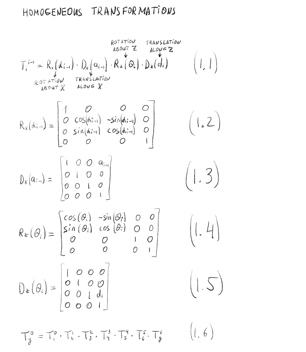
<p><img src="/imgs/robotics_projects/hom_transform_1000.png" alt="Forward Kinematics" />
<em>Forward Kinematics transform for Kuka KR210 Robotics Arm.</em></p>
<p>The whole derivation of forward and inverse kinematics with correction transforms and special cases of singularity you can find in my project write-up.</p>

<p>One might ask “Why do we need to bother with this math when ROS can give provide you all transformations through <code class="language-plaintext highlighter-rouge">tf</code> package?” I think it’s important to understand it all because:</p>
<ul>
  <li>ROS is not everywhere, and some systems can’t use it because of real-time requirements or sensitive applications</li>
  <li>There always new platforms and environments appearing so you sometimes need to write your implementation of things like linear algebra functions, forward and inverse kinematics calculations and SLAM algorithms (for example new ASICs or custom FPGA chips)</li>
</ul>

<p>I would also prefer to learn more about dynamics and mechanical parts, but it seems a vast topic and Udacity would probably need to launch a separate Robotics Hardware Nanodegree to cover it in a meaningful way.</p>

<p>Here is the links to my implementation of the project on <a href="https://github.com/bexcite/RoboND-Kinematics-Project">GitHub</a> and a <a href="https://github.com/bexcite/RoboND-Kinematics-Project/blob/master/writeup.md">write-up</a>.</p>

<p>Related links &amp; materials:</p>
<ul>
  <li><a href="https://www.youtube.com/watch?v=0yD3uBshJB0">Introduction to Robotics, Lectures 1-5 (CS223A)</a> in the Stanford Computer Science Department by Professor Oussama Khatib</li>
  <li><a href="https://pdfs.semanticscholar.org/188d/ca40fa862c5cd574f09ae68e1e4e30852fc5.pdf">Khatamian, A. (2015, January). Solving Kinematics Problems of a 6-DOF Robot Manipulator.</a></li>
  <li><a href="http://home.deib.polimi.it/gini/robot/docs/spong.pdf">Robot Dynamics and Control, by MW Spong</a></li>
</ul>

<h2 id="project-13-3d-perception">Project 1.3: 3D Perception</h2>

<p>What I like about Udacity’s course materials that they expose you to the real world problems and ongoing challenges in the robotics field.</p>

<p>Thus, the third project based on Amazon Robotics Challenge where the goal is to build a recognition pipeline for the set of known objects using RGB-D sensor data and send the correct pose for the robot to perform a pick-and-place operation.</p>

<p><img src="/imgs/robotics_projects/perception_robot.png" alt="Perception PR2 robot" /></p>

<p>Though that’s not enough for the participants because the full task for Amazon Robotics Challenge is to build an autonomous manipulator that can perform perception, motion planning, 3D mapping, kinematics and more to locate specific objects in cluttered dynamic environment retrieve and place them into a designated bin.</p>

<p>To train the model we need to collect point cloud data for each object in different orientations. Here is how Gazebo environment used for data collection by sequentially showing every object in random poses to the sensor and record HOG and surface normal feature vector.</p>

<p><img src="/imgs/robotics_projects/capture_features.gif" alt="Capture object features" /></p>

<p>It was excellent learning for me that with a quite simple 3D point cloud pipeline that goes through voxel downsampling, passthrough thresholding, RANSAC plane segmentation and Euclidean clustering we can separate individual points for objects on the table and apply SVM classifier to recognize them. Everything seems much complex in 3D than in 2D but this pipeline was clean, simple and produced great results (96% accuracy rate for SVM classifier).</p>

<p><img src="/imgs/robotics_projects/model3_1500_961.png" alt="SVM Classifier confusion matrix" />
<em>Confusion matrix for SVM Classifier</em></p>

<p><img src="/imgs/robotics_projects/perception_pipeline_1_opt.png" alt="3D Perception pipeline" />
<em>3D Perception pipeline: HOG &amp; Surface normals features + SVM Classifier</em></p>
<p>Look at my implementation of the project on <a href="https://github.com/bexcite/RoboND-Perception-Project">GitHub</a> and a <a href="https://github.com/bexcite/RoboND-Perception-Project/blob/master/writeup.md">write-up</a> link.</p>

<p>Related links &amp; materials:</p>
<ul>
  <li><a href="http://arc.cs.princeton.edu/">MIT-Princeton at the Amazon Robotics Challenge, Winner 2017</a></li>
  <li><a href="https://arxiv.org/abs/1703.09312">Mahler, Jeffrey, et al. “Dex-net 2.0: Deep learning to plan robust grasps with synthetic point clouds and analytic grasp metrics.”(2017).</a></li>
  <li><a href="https://arxiv.org/abs/1711.06396">Zhou, Yin, and Oncel Tuzel. “VoxelNet: End-to-End Learning for Point Cloud Based 3D Object Detection.” (2017).</a></li>
  <li><a href="https://www.youtube.com/watch?v=8CenT_4HWyY">CVPR 2017: Tutorial : 3D Deep Learning</a></li>
</ul>

<h3 id="project-14-follow-me">Project 1.4 Follow Me</h3>

<p>Well, that’s nice. If you are following drone industry updates, you probably know a couple of cases when drone companies claimed to build <em>“follow me”</em> feature and that drone be able to automatically fly beside you, take beautiful shots and avoid obstacles. Then they didn’t quite deliver on the promise because the task is just hard.</p>

<p>In this project, we’ve had a chance to build a part of this pipeline: person recognition through deep learning image segmentation and feed the data back to the drone simulator to test the following feature.</p>

<p>Udacity’s simulator is built on Unity game engine, and it’s an excellent tool as a playground for testing perception and control algorithms.</p>

<p><img src="/imgs/robotics_projects/follow_me_drone.png" alt="Follow Me Drone Simulator" />
<em>Udacity’s Drone Simulator</em></p>

<p>Image segmentation was build on Fully Connected Network (FCN) architecture that consists of convolutional encoder &amp; decoder. It’s the first architecture that you can start from and test other approaches like Mask R-CNN, for example.</p>

<p><img src="/imgs/robotics_projects/follow_me_network_fancy.png" alt="Deep Learning FCN" />
<em>Simple FCN architecture for image segmentation task</em></p>
<p>For the hero segmentation task with such an FCN I was able to get average IoU score <code class="language-plaintext highlighter-rouge">89.6%</code>.</p>

<p><img src="/imgs/robotics_projects/follow_me_example_1.png" alt="Deep Learning FCN" />
<em>Hero segmentation: Original image, Ground Truth, Segmentation Result</em></p>
<p>Here are links to my implementation of the project on <a href="https://github.com/bexcite/RoboND-DeepLearning-Project/blob/master/code/model_training.ipynb">GitHub</a> and a <a href="https://github.com/bexcite/RoboND-DeepLearning-Project/blob/master/writeup.md">write-up</a>.</p>

<p>Related links &amp; materials:</p>
<ul>
  <li><a href="https://www.cv-foundation.org/openaccess/content_cvpr_2015/app/2B_011.pdf">Long, J., Shelhamer, E., &amp; Darrell, T. (2015). Fully convolutional networks for semantic segmentation.</a></li>
  <li><a href="https://leonardoaraujosantos.gitbooks.io/artificial-inteligence/content/image_segmentation.html">Image Segmentation</a></li>
  <li><a href="http://openaccess.thecvf.com/content_cvpr_2017/papers/Pohlen_Full-Resolution_Residual_Networks_CVPR_2017_paper.pdf">Pohlen, Tobias, et al. “Full-resolution residual networks for semantic segmentation in street scenes.”(2017).</a></li>
  <li><a href="http://ieeexplore.ieee.org/abstract/document/8237584/">He, Kaiming, et al. “Mask r-cnn.”, 2017</a></li>
</ul>

<h3 id="project-21--robotic-inference">Project 2.1:  Robotic Inference</h3>

<p>In the first project of Term 2 we’ve explored the NVidia DIGITS system for training deep learning models for image classifications.</p>

<p>My choice was to build a model that can classify finger gestures so I can use it later for my home robots projects.</p>

<p>Data was collected manually using a camera on MacBook Pro.</p>

<p><img src="/imgs/robotics_projects/fingers_source_imgs_full1.png" alt="Fingers Classification Source Images" />
<em>Fingers Classification: Example dataset</em></p>

<p>Interestingly enough that LeNet was able to train and recognize fingers gesture with high accuracy and as a result the inference performance on Tesla K80 GPU was <code class="language-plaintext highlighter-rouge">0.19 ms</code>!</p>

<p>Details about the project and my implementation you can find in a previous article <a href="https://capsulesbot.com/blog/2018/02/02/classification-model-for-fingers-recognition.html">“Fingers Classification”</a> and the source code of supporting tools on <a href="https://github.com/bexcite/fingers_classification">GitHub</a>.</p>

<p>Related links:</p>
<ul>
  <li><a href="http://yann.lecun.com/exdb/lenet/">LeNet-5, convolutional neural networks</a></li>
  <li><a href="https://developer.nvidia.com/digits">NVidia DIGITS</a></li>
</ul>

<h3 id="project-22-where-am-i">Project 2.2: Where Am I?</h3>

<p>Here we are going deeper into a robot description and exploring Monte-Carlo Localization algorithm implementation in the ROS.</p>

<p>One part of the project is to build a robot model using URDF, test it in Gazebo and another is to configure localization stack using AMCL package.</p>

<p><img src="/imgs/robotics_projects/where_am_i_robot_solid.png" alt="Robot Model - URDF" /></p>

<p><em>Robot Model, with a laser scan and camera sensors</em></p>

<p>Current and future projects are teaching us to deal with dozens of parameters that you need to tune to make your system work. Robot model parameters – inertial, visual, collision; AMCL parameters – particles number, velocities limits, transform tolerance, odometry characteristics; Move Base parameters – inflation radius, robot footprint, local &amp; global cost map settings, planner settings and so on …</p>

<p>Sometimes it’s converging quickly, and you have a working robot, but sometimes it’s not, and you are moving circles making a lot of tweaks and tests launching ROS, RViz, and Gazebo many times.</p>

<iframe width="720" height="430" src="https://www.youtube.com/embed/qMKT9Q2fBQ0" frameborder="0" allow="autoplay; encrypted-media" allowfullscreen=""></iframe>
<p><em>My custom robot executing localization and navigation to the goal</em></p>

<p>Here are links to my implementation of the project on <a href="https://github.com/bexcite/udacity-bot">GitHub</a> and a <a href="https://github.com/bexcite/udacity-bot/blob/master/results/Where_Am_I_Report.pdf">write-up in PDF</a>.</p>

<p>Related links:</p>
<ul>
  <li><a href="http://robots.stanford.edu/papers/thrun.robust-mcl.pdf">Thrun, Sebastian, et al. “Robust Monte Carlo localization for mobile robots.” (2001).</a></li>
  <li><a href="https://docs.ufpr.br/~danielsantos/ProbabilisticRobotics.pdf">Thrun, Sebastian, Wolfram Burgard, and Dieter Fox. Probabilistic robotics. MIT press, 2005.</a></li>
</ul>

<h3 id="project-23-map-my-world-robot">Project 2.3: Map My World Robot</h3>

<p>It’s a SLAM project where we’ve explored different approaches to SLAM during the lessons: Full SLAM vs. Online SLAM, FastSLAM (EKF-based and Grid-based), GraphSLAM.</p>

<p><img src="/imgs/robotics_projects/map_my_world_slam_formulation.png" alt="SLAM problem formulation" />
<em>Durrant-Whyte et al. (2006)</em></p>

<p>We’ve used the mapping capabilities of <code class="language-plaintext highlighter-rouge">rtabmap</code> to map the environment using the previously build URDF robot model with a newly equipped depth camera and necessary configurations.</p>

<p>We’ve built the map of the provided environment and explored loop closure on the resulting map. Then we’ve modeled our environment in Gazebo and built the map for it with our configured robot using <code class="language-plaintext highlighter-rouge">rtabmap</code> implementation.</p>

<p><img src="/imgs/robotics_projects/map_my_world_lab_map_3d.png" alt="Rtabmap for custom environment 3D" /></p>

<p><em>3D map of custom environment. Built with <code class="language-plaintext highlighter-rouge">rtabmap</code>.</em></p>

<p>SLAM is very complex problem algorithmically and computationally, and it’s worth exploring it deeper because you can find it everywhere from AR/MR/VR headsets, controllers, mobile phones to self-driving cars and Mars rovers.</p>

<p>Here are links to my implementation of the project on <a href="https://github.com/bexcite/udacity_slam">GitHub</a> and a <a href="https://github.com/bexcite/udacity_slam/blob/master/slam_project/results/report_map_my_world.pdf">write-up in PDF</a>.</p>

<p>Related links:</p>
<ul>
  <li><a href="http://introlab.github.io/rtabmap/">Real-Time Appearance-Based Mapping</a></li>
  <li><a href="http://everobotics.org/pdf/SLAMTutorial.pdf">Durrant-Whyte, Hugh, and Tim Bailey. “Simultaneous localization and mapping: part I.” (2006).</a></li>
  <li><a href="http://ieeexplore.ieee.org/iel5/100/35300/01678144.pdf">Bailey, Tim, and Hugh Durrant-Whyte. “Simultaneous localization and mapping (SLAM): Part II.” (2006).</a></li>
  <li><a href="http://domino.informatik.uni-freiburg.de/teaching/ws10/praktikum/slamtutorial.pdf">Grisetti, Giorgio, et al. “A tutorial on graph-based SLAM.” (2010).</a></li>
</ul>

<h3 id="project-24-deep-rl-arm-manipulation">Project 2.4: Deep RL Arm Manipulation</h3>

<p>Deep Reinforcement Learning is the next big thing in deep learning, and you’ve probably heard about DeepMind, AlphaGo Zero or Open AI agent that plays Dota 2 tournaments against humans. This project is about an application of deep reinforcement learning to robotic tasks.</p>

<p>Objectives of the project were to create a DQN Agent and tune hyperparameters to achieve the two following tasks:</p>
<ol>
  <li>Any part of the robot arm should touch the object with at least an accuracy of 90%.</li>
  <li>Only the gripper base of the robot arm should touch the object with at least an accuracy of 80%.</li>
</ol>

<p>Project environment was built on ROS and Pytorch LSTM Network with C++ integrations to Gazebo plugin.</p>

<p><img src="/imgs/robotics_projects/deep_rl_task_2_result.png" alt="Deep RL Arm Manipulator results" />
<em>Deep RL Arm Manipulator trained for Task #2</em></p>
<p>The main difficulty in the project was to select the good reward function that would be able to learn the expected behaviors. I’ve spent more than <em>20 hours</em> of GPU’s compute time on Udacity Workspace on just training and testing different reward params.</p>

<p>Links to my implementation of the project on <a href="https://github.com/bexcite/RoboND-DeepRL-Project/tree/workspaces">GitHub</a> and a <a href="https://github.com/bexcite/RoboND-DeepRL-Project/blob/workspaces/report/Report_%20Deep%20RL%20Arm%20Manipulation.pdf">write-up in PDF</a>.</p>

<p>Relevant materials &amp; links:</p>
<ul>
  <li><a href="http://www0.cs.ucl.ac.uk/staff/d.silver/web/Teaching.html">David Silver Reinforcement Learning Lectures</a></li>
  <li><a href="https://github.com/dusty-nv/jetson-reinforcement">Dustin Franklin, Jetson TX2, Reinforcement Learning repo</a></li>
  <li><a href="https://blog.openai.com/dota-2/">Open AI: Dota 2</a></li>
  <li><a href="http://www.incompleteideas.net/book/bookdraft2018jan1.pdf">“Reinforcement Learning: An Introduction”, Richard S. Sutton and Andrew G. Barto, 2018</a></li>
</ul>

<h3 id="project-25-home-service-robot">Project 2.5: Home Service Robot</h3>

<p>Finally, I am returning to the project that was mentioned at the beginning of the article.</p>

<p>It’s an integration project to build the structure of home service robot that can build a map by executing a wall follower algorithm, navigate to the pick-up location, collect an object, navigate to the drop-off location and leave the object there.</p>

<p><img src="/imgs/robotics_projects/hs_goal1_complete.png" alt="Home Service Goal 1 Complete" />
<em>Home Service Robot completing Goal #1</em></p>

<p>Main challenges were to integrate everything in the ROS using and re-using packages from Turtlebot while implementing three custom nodes:</p>
<ul>
  <li>Add Markers</li>
  <li>Pick Objects</li>
  <li>Wall Follower</li>
</ul>

<p>Here the links to my implementation of the project on <a href="https://github.com/bexcite/udacity_hs">GitHub</a>.</p>

<p>Relevant materials &amp; links:</p>
<ul>
  <li><a href="https://www.turtlebot.com/">Turtlebot</a></li>
</ul>

<h2 id="future-work">Future work</h2>

<p>That was a great journey through the vast amount of information and tools. I’ve tried to break the ice of ROS and Gazebo myself 2 years ago but lost motivation without the task at hand and well-defined structure.</p>

<p>I think the primary value that you get from Udacity’s Nanodegree is the organized and straightforward success path for learning, projects tasks and environments that you can start playing with and community of like-minded people who are passionate about robotics and going through the challenges together with you.</p>

<p>My future work in the field would be:</p>
<ol>
  <li>Explore how one can make a higher order robotics sensor using open source and cheap hardware like Google Vision kit which has integrated Vision Bonnet board with Intel Movidius chipset – the great candidate for on the edge deep learning based processing.</li>
  <li>Build a 1/10 self-driving car model using Jetson TX2 + RC model and implement the navigation stack with some useful utility for a household.</li>
</ol>

<p>Happy learning and building autonomous robots.</p>

<p>PS: If you are in San Francisco - Bay Area, building robots or want to collaborate on some robotics/self-driving car projects I would be happy to chat with you.</p>]]></content><author><name>Pavlo Bashmakov</name></author><category term="blog" /><summary type="html"><![CDATA[My “home service” robot just finished dropping off the square marker and stopped in final position that was set as its second goal and executed by move_base ROS package that in turn uses the underlying navigation stack with global and local planners to build plan and eventually send commands to the controller that drives robot in simulation on Gazebo. That was the last requirement for the final project. I’ve tested it a bit more, prepared the archive with all ROS packages that contained custom nodes, configurations, scripts, launch files and send for the review.]]></summary></entry><entry><title type="html">MS Build 2018 Notes: Mixed Reality and Smart Enterprises</title><link href="/blog/2018/05/15/ms-build-notes-2018.html" rel="alternate" type="text/html" title="MS Build 2018 Notes: Mixed Reality and Smart Enterprises" /><published>2018-05-15T08:00:00+00:00</published><updated>2018-05-15T08:00:00+00:00</updated><id>/blog/2018/05/15/ms-build-notes-2018</id><content type="html" xml:base="/blog/2018/05/15/ms-build-notes-2018.html"><![CDATA[<p>I’ve spent four days on MS Build 2018 conference in Seattle and here my observations and thoughts. It’s not news though, and you can read/watch all announcements from MS Build 2018 somewhere on the Internet. Also please note that I’m probably biased towards one or another.</p>

<h2 id="general">General</h2>

<ol>
  <li>
    <p>Microsoft is very serious about <strong>2 Billion</strong> first <a href="https://www.forbes.com/sites/insights-microsoft/2018/01/25/6-challenges-of-empowering-firstline-workers-and-how-to-overcome-them/#54e7ec6118c3">line workers</a> and building solutions to tap into their workflows and processes.</p>
  </li>
  <li>
    <p>Once engaged into Microsoft stack businesses can’t stop but move forward integrating more and more Microsoft technology in their workflows.</p>
  </li>
  <li>
    <p>Microsoft has strong consultancy wing that builds custom enterprise solutions and helps grow the ecosystem of service providers who, in turn, integrate more and more Microsofts/Azure tech into enterprises.</p>
  </li>
  <li>
    <p>Microsoft helps integrators and agencies only when they bring substantial value to Microsoft itself - big customer that uses Azure products, or great use case with enterprise customer that they can make case study or video about it, etc. (though it’s like every other company)</p>
  </li>
  <li>
    <p>There wasn’t much mobile news anymore; it’s just a platform where users should have access to Microsoft Graph, Microsoft Teams, Office 365, Azure Cognitive Services and interact with new platforms like Mixed Reality.</p>
  </li>
  <li>
    <p>I am (almost) complete stranger in Microsoft Ecosystem (and still is), but I see big enterprises are there, ecosystem is there, and Microsoft’s pace of innovation is on par and in some spaces even better than Amazon, Facebook, Google, Apple (consider AI stuff, HoloLens and Microsoft Graph).</p>
  </li>
</ol>

<p>As a conclusion, Amazon AWS and Microsoft Azure (+ everything else in MS stack) is the great place to be for any consultancy and service business if they want to work with big enterprises, but MS looks like a hard die for everyone who doesn’t have previous experience with MS products and switched long time ago to all Mac/Linux paradigm. However, MS is closing this gaps with an introduction of Linux shell support and event Notepad support Unix style line endings :)</p>

<h2 id="cloud--edge">Cloud &amp; Edge</h2>

<ol>
  <li>
    <p>Everyone is migrating to the cloud, from on-premise and privately owned data centers. It started occurring 3-5 years ago within enterprises and will be continuing further. More data are coming to companies more migration efforts needed in the future. (Just copying petabytes of data is not an easy endeavor).</p>
  </li>
  <li>
    <p>More data leads to more requests in data analysis and AI infrastructure needs to retrieve and process data. And more opportunities for services based on Microsoft Graph and Spatial Analytics to provide value for customers.</p>
  </li>
  <li>
    <p>Cortana will be on par with <a href="https://ai.googleblog.com/2018/05/duplex-ai-system-for-natural-conversation.html">Google’s Duplex</a> in 2-3 years but for enterprises. Make chores like meeting confirmations, reminders, gathering information according to the brief or soliciting requirements.</p>
  </li>
  <li>
    <p>It will help with meetings and execution of mundane tasks in companies from travel arrangements to customer research. Outlook once killed assistants’ job and Cortana powered with Microsoft Graph will free time and boost productivity for accountants, lawyers, event managers and HR specialists.</p>
  </li>
  <li>
    <p>Real-time is hard, and MS is continuing moving inference and data processing to the edge. It’s playing a card of smart factories and enterprises. I think this is a huge market where technology can add substantial value to real-world problem like making factory floors safer, more predictable and satisfying.</p>
  </li>
  <li>
    <p>Containers and Kubernetes are everywhere in web dev, in AI/ML, IoT, etc. It’s like the new standard in software engineering.</p>
  </li>
</ol>

<h2 id="cognitive-services---ai-nlp-vision-audio-etc">Cognitive Services - AI, NLP, Vision, Audio, etc</h2>

<ol>
  <li>
    <p>MS strong in AI API’s, algorithms and they are not losing their pace. We can expect more intelligence in NLP and vision (especially for enterprise tasks - manufacturing, factory floor, drones, etc.)</p>
  </li>
  <li>
    <p>~25 AI services are available and easy to train and use. And now they are even available as a function in Excel connected to the whole Azure infrastructure and DBs.</p>
  </li>
  <li>
    <p>Microsoft’s research in AI and FPGA based hardware are strong. You can easily encounter on their papers ranging from NLP to 3D pose tracking with the state-of-the-art results and datasets.</p>
  </li>
  <li>
    <p>Sensors + Software + Hardware + Cloud we can see this formula is unrolling in <a href="https://azure.microsoft.com/en-us/campaigns/kinect/">Project Kinect for Azure</a> and Spatial Analytics Audio device that they showcased on expo floors.</p>
  </li>
</ol>

<h2 id="mixed-reality---arvr-on-microsofts-terms">Mixed Reality - AR/VR on Microsofts Terms</h2>

<ol>
  <li>
    <p>Thousands of people are working on Mixed Reality in Microsoft. It’s a big bet for them and they are leading the innovation here with a) HoloLens and b) Project Kinect for Azure sensors.</p>
  </li>
  <li>
    <p>It wasn’t directly confirmed but all signs that MS is working on HoloLens v2. We can expect more computational power, better tracking with new Kinect sensors hardware and integrated collaboration services like Microsoft Assist and Microsoft Teams. (speculation)</p>
  </li>
  <li>
    <p>Mixed Reality is for collaboration and shared experiences.</p>
  </li>
  <li>
    <p>While Amazon and Google are building connected homes, MS is building connected offices, factory floors, and warehouses.</p>
  </li>
  <li>The most popular use cases for MR in enterprises are:
    <ul>
      <li>Training</li>
      <li>Remote assistance (integrated with companies system and processes)</li>
      <li>Design together (car design etc.)</li>
    </ul>
  </li>
  <li>Almost all manufacturing is dealing with CAD and 3D models, and they want all their processes to be organized around 3D models. Any system should support and work on all platforms - PC, Web, Mobile and VR/AR headsets now.</li>
</ol>

<h2 id="collaboration-epos">Collaboration <em>epos</em></h2>

<ol>
  <li>
    <p>Everything always was around people and collaboration. Hence avatars, multi-player, body/faces expression/eyes tracking, etc.</p>
  </li>
  <li>
    <p>All services and media are about the collaboration of people with other people. In MR, in chats, in training and remote assistance, and so on and so on.</p>
  </li>
</ol>

<h2 id="spatial-analytics-sensors--enterprises">Spatial Analytics: Sensors &amp; Enterprises</h2>

<ol>
  <li>
    <p>MS is pushing forward with the vision of <a href="https://www.youtube.com/watch?v=pL-c00M2CnI&amp;t=32s">smart connected floor</a> that continuously tracks everything and provides back insights and analytics.</p>
  </li>
  <li>
    <p>Spatial Analytics: Audio Array + Project Azure Kinect (the best in class depth sensor) + Smart Camera with on the edge processing. All this will be glued together with dedicated smart Azure services in 1-2 years.</p>
  </li>
  <li>
    <p>Cortana + Spatial Analytics “feelings” and we have a factory supervisor like intelligent spaceship “Justice of Toren” from <a href="https://en.wikipedia.org/wiki/Ancillary_Justice">“Ancillary Justice”</a>.</p>
  </li>
</ol>

<h2 id="blockchain">Blockchain</h2>

<ol>
  <li>Yep, Azure has <a href="https://azure.microsoft.com/en-us/solutions/blockchain/">blockchain services</a> ready for enterprise integrations.</li>
</ol>

<h2 id="summary">Summary</h2>

<p>Vision is easy; execution is much-much harder. Switch gears and tap into execution and delivery of real systems and solutions that work for enterprises of the future.</p>]]></content><author><name>Pavlo Bashmakov</name></author><category term="blog" /><summary type="html"><![CDATA[I’ve spent four days on MS Build 2018 conference in Seattle and here my observations and thoughts. It’s not news though, and you can read/watch all announcements from MS Build 2018 somewhere on the Internet. Also please note that I’m probably biased towards one or another.]]></summary></entry><entry><title type="html">Train Fingers Classification Model Using NVidia DIGITS</title><link href="/blog/2018/02/02/classification-model-for-fingers-recognition.html" rel="alternate" type="text/html" title="Train Fingers Classification Model Using NVidia DIGITS" /><published>2018-02-02T08:00:00+00:00</published><updated>2018-02-02T08:00:00+00:00</updated><id>/blog/2018/02/02/classification-model-for-fingers-recognition</id><content type="html" xml:base="/blog/2018/02/02/classification-model-for-fingers-recognition.html"><![CDATA[<p>NVidia DIGITS is a simple and useful integration of deep learning framework Caffe into the cloud settings. I’ll use it for my pet project of fingers recognition trained end-to-end. Resulting model can be easily loaded to a mobile robot powered on Jetson TX2 but let’s leave it for another post.</p>

<h2 id="introduction">Introduction</h2>

<p>Mobile robots need to sense the world around and reason about it. Different sensors convey different modality on which we are building perception, control, localization, mapping and behavioral planning. Visual perception is the key to a robot perception system due to high information density that images contain. Though images were always difficult to process both algorithmically and computationally. With the advances in deep learning and GPU computing chips, we can easily build end-to-end systems for a specific task with the fraction of efforts that we needed a decade ago.</p>

<p>Gestures is a natural human interaction method that we can apply for mobile robot control. Different systems of hand-gestures mobile robots control was proposed: image pre-processing and feature of extraction state <a href="#references">[1]</a>, wearable inertial-sensor-based system <a href="#references">[3]</a>, system based on hidden markov models <a href="#references">[4]</a>, or neural networks EOG gesture recognition <a href="#references">[5]</a>.</p>

<p>Here I am exploring the end-to-end system for gesture recognition that was trained on a manually collected dataset and using an NVidia DIGITS for training.</p>

<h2 id="data-acquisition-and-pre-processing">Data Acquisition and Pre-processing</h2>

<p>Data was manually collected using a MacBook Pro built-in camera and a python script <code class="language-plaintext highlighter-rouge">grab_images.py</code>. All script sources are available on my Github repo <a href="https://github.com/bexcite/fingers_classification">bexcite/fingers_classification</a>.</p>

<div class="language-plaintext highlighter-rouge"><div class="highlight"><pre class="highlight"><code>python grab_images.py --size 28 --rate 10 --gray
</code></pre></div></div>

<p>It captures frames at 10 Hz <code class="language-plaintext highlighter-rouge">rate</code>, resizes it to 28x28 (<code class="language-plaintext highlighter-rouge">resize</code>), and saves in a grayscale <code class="language-plaintext highlighter-rouge">gray</code>.</p>

<p>Different lighting conditions, backgrounds variations, angles of the gestures and spatial rotations were used to cover the broad spectrum of possible uses.</p>

<p>Additional data augmentation was used to flip images horizontally to additionally increase the dataset and variations. (<a href="https://github.com/bexcite/fingers_classification">source</a>)</p>

<div class="language-plaintext highlighter-rouge"><div class="highlight"><pre class="highlight"><code>python augment_images.py --input_dir &lt;data&gt; --output_dir &lt;aug_data&gt; --resize 28
</code></pre></div></div>

<p>Below is an example of images collected before resizing.</p>

<p><img src="/imgs/classification_model_fingers/fingers/source_imgs_full1.png" alt="Fingers original" /></p>

<p>Examples of processed images that were used during the training (scaled for the better view).</p>

<p><img src="/imgs/classification_model_fingers/fingers/source_imgs_gray_full1.png" alt="Fingers processed" /></p>

<h2 id="formulation-and-model-training">Formulation and Model Training</h2>

<p>Fingers recognition for the mobile robot should be as fast as possible and don’t take computer time from control and localization pipelines. I’ve tested two ready-made networks in DIGITS, LeNet and GoogLeNet, with the fastest results and good accuracy achieved on a standard LeNet convolutional network with gray images of size 28x28 pixels.</p>

<p><img src="/imgs/classification_model_fingers/fingers/lenet_arch.png" alt="LeNet Architecture" /></p>

<p>Network converged after around 10 epochs in a matter of seconds.</p>

<p><img src="/imgs/classification_model_fingers/fingers/fingers_training_loss_accuracy.png" alt="Fingers training" /></p>

<p>It was trained using SGD with the starting learning rate 0.01 and a scheduled decrease.</p>

<p><img src="/imgs/classification_model_fingers/fingers/fingers_learning_rate.png" alt="Fingers training" /></p>

<h2 id="results">Results</h2>

<p>Fingers dataset trained on LeNet network showed the good accuracy for all classes and inference speed <code class="language-plaintext highlighter-rouge">0.19ms</code> on a Tesla K80 GPU.</p>

<p>Below is the result output from TensorRT for inference speed evaluation:</p>

<p><img src="/imgs/classification_model_fingers/fingers/fingers_results_clean.png" alt="Fingers results" /></p>

<p>Confusion matrix for a test dataset:</p>

<p><img src="/imgs/classification_model_fingers/fingers/fingers_confusion.png" alt="Fingers confusion matrix" /></p>

<h2 id="discussion">Discussion</h2>

<p>It was unexpected that LeNet and 28x28 gray images of 6 possible combinations of fingers gesture could produce acceptable results. Though if we look closer into 28x28 images of training dataset, it becomes clear that it’s possible to recognize the depicted gesture and amount of fingers in almost all images so convolutional layers were able to extract the meaningful features too.</p>

<h2 id="next">Next</h2>

<p>Next I’m planning to load this network on Jetson TX2 and see how it performs in real-time on smaller hardware so eventually my robot could recognize hand gesture commands while navigating around an apartment.</p>

<h2 id="references">References</h2>

<ol>
  <li>
    <p>Ali, Muaammar Hadi Kuzman, M. Asyraf Azman, and Zool Hilmi Ismail. “Real-time hand gestures system for mobile robots control.” Procedia Engineering 41 (2012): 798-804. <a href="https://www.sciencedirect.com/science/article/pii/S187770581202646X">link &gt;</a></p>
  </li>
  <li>
    <p>Manigandan, Mr, and I. Manju Jackin. “Wireless vision based mobile robot control using hand gesture recognition through perceptual color space.” Advances in Computer Engineering (ACE), 2010 International Conference on. IEEE, 2010. <a href="http://ieeexplore.ieee.org/document/5532868/">link &gt;</a></p>
  </li>
  <li>
    <p>Stančić, Ivo, Josip Musić, and Tamara Grujić. “Gesture recognition system for real-time mobile robot control based on inertial sensors and motion strings.” Engineering Applications of Artificial Intelligence 66 (2017): 33-48. <a href="https://www.sciencedirect.com/science/article/pii/S0952197617301975">link &gt;</a></p>
  </li>
  <li>
    <p>Iba, Soshi, et al. “An architecture for gesture-based control of mobile robots.” Intelligent Robots and Systems, 1999. IROS’99. Proceedings. 1999 IEEE/RSJ International Conference on. Vol. 2. IEEE, 1999. <a href="http://www.cs.cmu.edu/~cyberscout/publications/IROS99_GBC.pdf">link &gt;</a></p>
  </li>
  <li>
    <p>SASAKI, Minoru, and Yanagido Gifu. “Mobile Robot Control by Neural Networks EOG Gesture Recognition.” <a href="http://citeseerx.ist.psu.edu/viewdoc/download?doi=10.1.1.494.5976&amp;rep=rep1&amp;type=pdf">link &gt;</a></p>
  </li>
  <li>
    <p>Sabour, Sara, Nicholas Frosst, and Geoffrey E. Hinton. “Dynamic routing between capsules.” Advances in Neural Information Processing Systems. 2017. <a href="https://arxiv.org/abs/1710.09829v1">link &gt;</a></p>
  </li>
  <li>
    <p>LeCun, Yann, et al. “Gradient-based learning applied to document recognition.” Proceedings of the IEEE 86.11 (1998): 2278-2324. <a href="http://yann.lecun.com/exdb/publis/pdf/lecun-98.pdf">link &gt;</a></p>
  </li>
</ol>]]></content><author><name>Pavlo Bashmakov</name></author><category term="blog" /><summary type="html"><![CDATA[NVidia DIGITS is a simple and useful integration of deep learning framework Caffe into the cloud settings. I’ll use it for my pet project of fingers recognition trained end-to-end. Resulting model can be easily loaded to a mobile robot powered on Jetson TX2 but let’s leave it for another post.]]></summary></entry><entry><title type="html">Low Earth Orbit (LEO) and delta-V requirements</title><link href="/blog/2018/01/21/low-earth-orbit-and-delta-v.html" rel="alternate" type="text/html" title="Low Earth Orbit (LEO) and delta-V requirements" /><published>2018-01-21T08:00:00+00:00</published><updated>2018-01-21T08:00:00+00:00</updated><id>/blog/2018/01/21/low-earth-orbit-and-delta-v</id><content type="html" xml:base="/blog/2018/01/21/low-earth-orbit-and-delta-v.html"><![CDATA[<p>Outer space starts at 100 km altitude (Karman line) where the atmosphere is so thin that it’s no longer provide aerodynamic lift and objects need to travel faster than orbital velocity to support itself.</p>

<p>Low Earth Orbit (LEO) starts around 160 km and up to 2,000 km. Below 160 km atmospheric drag is so strong that objects are quickly losing speed, so orbit is rapidly decaying.</p>

<p>To stay long enough on LEO without decaying objects needs to use some propulsion to boost their speed periodically. For example, ISS reboosting itself a couple of times per year.</p>

<p>Delta-v requirements to reach Low Earth Orbits starts approximately at 9.4 km/s.</p>

<p><img src="/imgs/low_earth_orbit/Orbital_low_1300.png" alt="Low Earth Orbit" /></p>]]></content><author><name>Pavlo Bashmakov</name></author><category term="blog" /><summary type="html"><![CDATA[Outer space starts at 100 km altitude (Karman line) where the atmosphere is so thin that it’s no longer provide aerodynamic lift and objects need to travel faster than orbital velocity to support itself.]]></summary></entry><entry><title type="html">Links to my 7 older posts (2015)</title><link href="/blog/2017/12/24/older-posts.html" rel="alternate" type="text/html" title="Links to my 7 older posts (2015)" /><published>2017-12-24T08:00:00+00:00</published><updated>2017-12-24T08:00:00+00:00</updated><id>/blog/2017/12/24/older-posts</id><content type="html" xml:base="/blog/2017/12/24/older-posts.html"><![CDATA[<p>Up until now, there wasn’t one place where I can collect all my articles. Here I’ve collected links to some old blog posts that I wrote elsewhere until Dec 2017 (and which are still alive, some gone extinct under domains/sites that no longer available)</p>

<p><a href="https://medium.com/mobile-design-and-ux/smartwatch-user-interaction-39601215a1b1">Smartwatch User Interaction (2015)</a> —
How users interact with a smartwatch and what UI components do they use</p>

<p><a href="https://medium.com/stanfy-engineering-practices/pros-and-cons-of-using-embedded-android-for-a-non-mobile-device-4fb3d2634a3b">Pros and Cons of Using Embedded Android for a Non-Mobile Device (2015)</a></p>

<p><a href="https://medium.com/@bashmakov/why-your-startup-needs-a-cross-functional-team-to-be-successful-cc40c905e730">Why Your Startup Needs a Cross-functional Team to be Successful (2015)</a></p>

<p><a href="https://medium.com/@bashmakov/slack-native-advertising-bot-a2d99fba9692">Slack Native Advertising Bot (2015)</a> — how ads might look like in our chats</p>

<p><a href="https://medium.com/stanfy-engineering-practices/3-types-of-software-architecture-for-connected-devices-a-smart-light-bulb-case-54dc7727136f">3 Types of Software Architecture for Connected Devices (2015)</a> — A Smart Light Bulb Case</p>

<p><a href="https://medium.com/inside-stanfy/what-we-ve-learned-from-10-years-of-being-in-the-software-development-business-f2547bf0e901">What we’ve learned from 10 years of being in the software development business (2015)</a></p>

<p><a href="https://medium.com/inside-stanfy/we-need-more-virtual-reality-content-4eed95e6a1fb">We need more Virtual Reality content (2015)</a> — It is the future of display technology.</p>]]></content><author><name>Pavlo Bashmakov</name></author><category term="blog" /><summary type="html"><![CDATA[Up until now, there wasn’t one place where I can collect all my articles. Here I’ve collected links to some old blog posts that I wrote elsewhere until Dec 2017 (and which are still alive, some gone extinct under domains/sites that no longer available)]]></summary></entry></feed>