Lidar odometry smoothing using ES EKF and KissICP for Ouster sensors with IMUs
In this post I’ve explored the possibility of improving the KissICP trajectory output for Ouster Lidars using the sensor’s embedded IMUs. On some environments ES EKF filtering together with KissICP made the 10% decrease in the ATE for high resolution 128 beam sensors but on other environments with lower resolution 32 beam sensors it showed 50% decrease in ATE compared to ground truth. ES EKF filter formulation and experiments described with references, source code and CLI tools for visualizations that may be used to replicate and test approaches on any Ouster’s Lidar pcap/bag raw data recordings.
Motivation and Related works
Since Ouster Lidar has an embedded IMU with time synchronization with lidar scans it should be beneficial to utilize it for Lidar based odometry and, possibly, reduce the drift, avoid system degradation on feature-less environments and improve results in fast movement scenarios.
As a good starting point to review the current state of Lidar based odometry and different approaches you can check this “LiDAR Odometry Survey [1]“.
In my experiment I will extend on the KissICP [2] implementation since it’s already tested with Ouster sensors and it’s SDK [3]. The main test dataset used for experiments is Newer College Dataset 2021 extension [4] with OS-0 128 beam sensor and latest Ouster sensors sample raw data recordings [5]
Overall system description
The input to the system is an Ouster lidar raw sensor data in the form of UDP packets payload from pcap/bag container.
ES EKF performs state prediction and error-state tracking on every incoming IMU measurement. When the new scan is available KissICP registers it, optionally using the ES EKF state as the initial pose guess, and the resulting pose used for the ES EKF update step. The output of the system is the ES EKF state which is the smoothed trajectory, see Fig. 1 below.
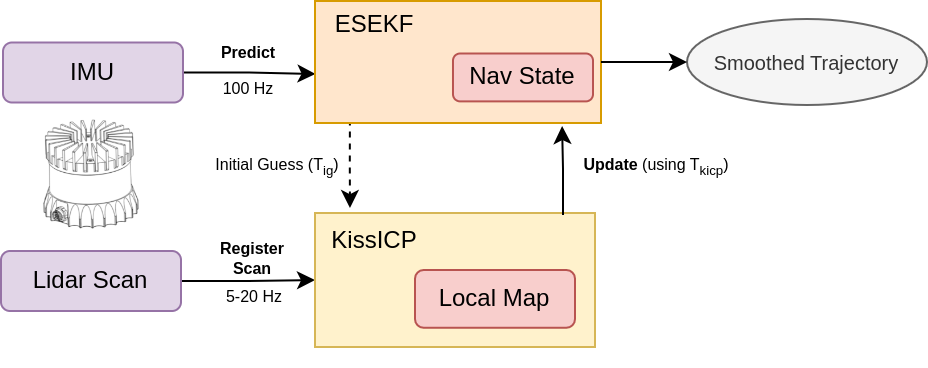
NOTE: Even though the imu packets and lidar packets is the Ouster wire data format and the pipeline works with live sensors too one should make additional efforts to tune the setup for the specific system performance which depends on machine setup (compute, memory, network), sensor resolution (32, 64 or 128 beams), KissICP parameters (internal map size, downsampling ratios, etc.) and sensor configuration (lidar mode, lidar profile, etc).
ES EKF: Error-state Extended Kalman Filter formulation
The main effect of the ES EKF contribution to the pipeline is to integrate the available IMU information and fuse it with the KissICP trajectory output while also providing the better initial guess for the point cloud registration step.
The exposition of the ES EKF below is very brief and more like to provide the overall structure of what is inside with the references to other sources with fully detailed derivations, possible modifications to update steps, etc. I heavily relied on the work “Quaternion kinematics for the error-state Kalman filter” by Joan Sola [6] where the Error-state EKF derivations and formulations were cleanly presented for the quaternions but could be easily adopted for the exponential representations.
Other important sources: in-depth IMU mechanisations for low-cost sensors could be found in [7], Kalman filters modular design approaches [8], multi sensor data fusion [9] and useful background theory and results on Lie Groups for 3D [10, 11, 12]
Predict step using new IMU measurement
The nominal filter state is defined as the following:
\[\boldsymbol{x} = \{ \boldsymbol{t}, \boldsymbol{v}, \boldsymbol{R}, \boldsymbol{b_g}, \boldsymbol{b_a} \}\]where $\boldsymbol{t},\boldsymbol{v} \in \mathbb{R}^{3}$ are the position and velocity in global frame, $\boldsymbol{R} \in SO(3)$ (or alternatively $\boldsymbol{q} \in \mathbb{H}$ can be used) is a rotation in global frame (as a rotation matrix or quaternion) and $\boldsymbol{b_g}, \boldsymbol{b_a} \in \mathbb{R}^{3}$ are gyroscope and accelerometer biases to be estimated.
Nominal state discrete-time kinematics, i.e. predict step that happens on every new IMU measurement:
\[\begin{aligned} \boldsymbol{\tilde{t}_k} & = t_{k-1} + v_{k-1} \Delta{t} + \frac{1}{2}(R_{k-1}(a_k - b_{a,k-1}) + \boldsymbol{g})\Delta{t}^2 \\ \boldsymbol{\tilde{v}_k} & = v_{k-1} + (R_{k-1}(a_k - b_{a,k-1}) + \boldsymbol{g})\Delta{t} \\ \boldsymbol{\tilde{R}_k} & = R_{k-1} Exp((\omega_k - b_{g,k-1})\Delta{t})) \\ \boldsymbol{\tilde{b}_{g,k}} & = b_{g,k-1} \\ \boldsymbol{\tilde{b}_{a,k}} & = b_{a,k-1} \end{aligned}\]Let’s define the nominal state evolved during the IMU prediction step as $\boldsymbol{\tilde{x}_k}$.
The error-state is defined as following:
\[\boldsymbol{\delta{x}} = \{ \boldsymbol{\delta{t}}, \boldsymbol{\delta{v}}, \boldsymbol{\delta{\phi}}, \boldsymbol{\delta{b_g}}, \boldsymbol{\delta{b_a}} \}\]where $\boldsymbol{\delta{t}}, \boldsymbol{\delta{v}}, \boldsymbol{\delta{\phi}} \in \mathbb{R}^3$ is the position, velocity and rotation errors, $\boldsymbol{\delta{b_g}}, \boldsymbol{\delta{b_a}} \in \mathbb{R}^3$ is the bias errors of gyroscope and accelerometer.
Error-state is evolving together with a nominal state in-between the update steps on IMU measurements and its kinematics in discrete-time:
\[\begin{aligned} \boldsymbol{\delta{t}_k} & = \delta{t}_{k-1} + \delta{v}_{k-1} \Delta{t} \\ \boldsymbol{\delta{v}_k} & = \delta{v}_{k-1} + (-R_{k-1}[\mathbf{a}_k - b_{a, k-1}]_{\times}\delta{\phi}_{k-1} - R_{k-1}\delta{b_{a,k-1}})\Delta{t} + \mathbf{v_i} \\ \boldsymbol{\delta{\phi}_k} & = Exp((\mathbf{\omega}_k - b_{g, k-1})\Delta{t})^{T}\delta{\phi}_{k-1} - \delta{b_{g, k-1}}\Delta{t} + \mathbf{\phi_i} \\ \boldsymbol{\delta{b_{g, k}}} & = \delta{b_{g, k-1}} + \mathbf{\omega_i} \\ \boldsymbol{\delta{b_{a, k}}} & = \delta{b_{a, k-1}} + \mathbf{a_i} \end{aligned}\]where $\mathbf{v_i}, \mathbf{\phi_i}, \mathbf{\omega_i}$ and $\mathbf{a_i}$ are the random impulses modeled as white Gaussian processes. Integrating the corresponding covariances of accelerometer/gyriscope biases and random walks we obtain the noise covariance matrices:
\[\begin{aligned} \boldsymbol{V_i} & = \sigma_{a_n}^2 \Delta{t}^{2} \boldsymbol{I} \\ \boldsymbol{\Phi_i} & = \sigma_{\omega_n}^2 \Delta{t}^{2} \boldsymbol{I} \\ \boldsymbol{\Omega_i} & = \sigma_{\omega_w}^2 \Delta{t} \boldsymbol{I} \\ \boldsymbol{A_i} & = \sigma_{a_w}^2 \Delta{t} \boldsymbol{I} \end{aligned}\]Introducing the input signal vector, from IMU measurement, and random process impulses vector as $\boldsymbol{u_k} = [a_k, \omega_k]^T$, $\boldsymbol{i} = [\boldsymbol{v_i}, \boldsymbol{\phi_i}, \boldsymbol{a_i}, \boldsymbol{\omega_i}]^T$ the error-state system can be written as:
\[\boldsymbol{\delta{x}_k} \leftarrow f(\boldsymbol{\tilde{x}_{k-1}}, \boldsymbol{\delta{x_{k-1}}}, \boldsymbol{u_k}, \boldsymbol{i}) = F_x(\boldsymbol{x_{k-1}}, \boldsymbol{u_k}) \delta{x} + F_i \boldsymbol{i}\]ES EKF predict step equations then (for error-state mean $\boldsymbol{\delta_x} \in \mathbb{R}^{15}$ and process covariance $\boldsymbol{P} \in \mathbb{R}^{15 \times 15}$ estimates):
\[\begin{aligned} \boldsymbol{\delta{x}_k} & = F_x(\boldsymbol{x_{k-1}}, \boldsymbol{u_k}) \delta{x} \\ \boldsymbol{P_k} & = F_x \boldsymbol{P_{k-1}} F_{x}^T + F_i \boldsymbol{Q_i} F_{i}^T \end{aligned}\]In expressions above $F_x$ is a Jacobian of the error-state transition function at the current point $\boldsymbol{x}_k, \boldsymbol{u_k}$ and can be written as:
\[F_x = \frac{\partial{f}}{\partial{\delta{x}}}\bigg|_{x_{k-1}, u_k} = \begin{bmatrix} \boldsymbol{I} && \boldsymbol{I} \Delta{t} && 0 && 0 && 0 \\ 0 && \boldsymbol{I} && -R_{k-1}[\mathbf{a}_k - b_{a, k-1}]_{\times}\Delta{t} && 0 && - R_{k-1}\Delta{t} \\ 0 && 0 && Exp((\mathbf{\omega}_k - b_{g, k-1})\Delta{t})^{T} && - \boldsymbol{I}\Delta{t} && 0 \\ 0 && 0 && 0 && \boldsymbol{I} && 0 \\ 0 && 0 && 0 && 0 && \boldsymbol{I} \end{bmatrix}\]and $F_i$ is a Jacobian with respect to random impulses $\boldsymbol{i}$ which can be written as:
\[F_i = \frac{\partial{f}}{\partial{\boldsymbol{i}}}\bigg|_{x_{k-1}, u_k} = \begin{bmatrix} 0 && 0 && 0 && 0 \\ \boldsymbol{I} && 0 && 0 && 0 \\ 0 && \boldsymbol{I} && 0 && 0 \\ 0 && 0 && \boldsymbol{I} && 0 \\ 0 && 0 && 0 && \boldsymbol{I} \end{bmatrix} \,, \quad Q_i = \begin{bmatrix} \boldsymbol{V_i} && 0 && 0 && 0 \\ 0 && \boldsymbol{\Phi_i} && 0 && 0 \\ 0 && 0 && \boldsymbol{\Omega_i} && 0 \\ 0 && 0 && 0 && \boldsymbol{A_i} \end{bmatrix}\]Update step using KissICP pose
KissICP registers every lidar frame, with optional initial guess pose obtained from the ES EKF filter, and returns the new system pose $z_k = T_{kicp, k} = [ R_{kicp, k} \, \vert \, t_{kicp, k} ]$ which then used in the update state of the filter.
The measurement model $h(\hat{x}_k)$ that is using the best true-state at the time of update $\hat{x}_k = \tilde{x} \oplus \delta{x}_k$ is:
\[h(\hat{x}_k) = h(\tilde{x} \oplus \delta{x}_k) = [ \tilde{R}_k Exp(\delta{\phi}_k) \, \vert \, \tilde{t}_k + \delta{t}_k ]\]The Jacobian $H$ of the measurement model with respect to the error-state $\delta{x}$ is defined as:
\[H = \frac{\partial{h}}{\partial{\delta{x}}} \bigg|_x = \begin{bmatrix} \boldsymbol{I} && 0 && 0 && 0 && 0 \\ 0 && 0 && \boldsymbol{I} && 0 && 0 \end{bmatrix} \quad \in \mathbb{R}^{6 \times 15}\]The measurement residual thus is:
\[y_k = z_k \ominus h(\hat{x}) = \begin{bmatrix} t_{kicp,k} - \tilde{t}_k - \delta{t}_k \\ Log(Exp(\delta{\phi}_k)^T \tilde{R}_k^T R_{kicp, k}) \end{bmatrix} \, \in \mathbb{R}^{1 \times 6}\]Now the complete set of equations for the ES EKF update step can be expressed as:
\[\begin{aligned} S & = H \boldsymbol{P}_{k-1} H^T + \boldsymbol{V} \\ K & = \boldsymbol{P}_{k-1} H^T S^{-1} \\ \delta{x}_k & \leftarrow K y_k \\ \boldsymbol{P}_k & \leftarrow (\boldsymbol{I} - K H) \boldsymbol{P}_{k-1} \end{aligned}\]where $\boldsymbol{V} \in \mathbb{R}^{6 \times 6}$ is the measurement error covariances of pose translation and pose rotation, which highly depends on the sensor used and it’s accuracy specs.
Inject the error into nominal state and reset the error-state
After we’ve got a KissICP pose $T_{kicp,k}$ estimate and updated the error-state mean $\delta{x}_k$ and covariance $P_k$ we need to incorporate the error-state into nominal state $\boldsymbol{x}_k = \tilde{x}_k \oplus \delta{x}_k$, or in expanded form:
\[\begin{aligned} \boldsymbol{t}_k & = \tilde{t}_k + \delta{t}_k \\ \boldsymbol{v}_k & = \tilde{v}_k + \delta{v}_k \\ \boldsymbol{R}_k & = \tilde{R}_k Exp(\delta{\phi}_k) \\ \boldsymbol{b}_{g,k} & = \tilde{b}_{g,k} + \delta{b}_{g,k} \\ \boldsymbol{b}_{a,k} & = \tilde{b}_{a,k} + \delta{b}_{a,k} \end{aligned}\]Then we reset the error-state $\delta{x} \leftarrow 0$ and ready to receive the new IMU measurements and execute predict step and so on.
Covariance $\boldsymbol{P}$ maybe left unchanged on the reset step or corrected to decrease the long-term error and odometry drift, please refer to [6], eqns 285-287 for details and derivations of such covariance correction.
Experimental results
The ES EKF implementation was done as part of the ptudes ekf-bench (Point eTudes) playground with metrics visualization, ground truth comparison (with ATE calculations) and point cloud visualization (with flyby viz for qualitative reviews). Newer College Dataset 2021 [4] extension was used to compare the results with ground truth.
Simulated IMU data or direct GT poses
The basic operation of ES EKF was validated with simulated IMU with/without noise that can be compared to the dead reckoning INS in the absence of the accelerometer/gyroscope noise and biases and using the ground truth poses as a correction input to check the filter convergence (see ptudes ekf-bench sim and ptudes ekf-bench nc commands correspondingly).
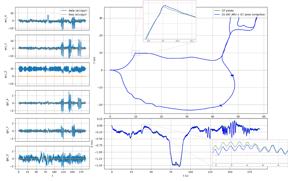
ptudes ekf-bench nc)The ES EKF performance of tracking the IMU inputs with direct ground truth poses as an update on the collection1/quad-hard sequence of the Newer College 2021 Dataset shown on Fig. 2 above, the Average Trajectory Errors (ATE) for position and rotation resulting in 0.0007 m and 0.0004 deg correspondingly (see [13] for ATE calculations details).
Ouster Lidar data with IMU
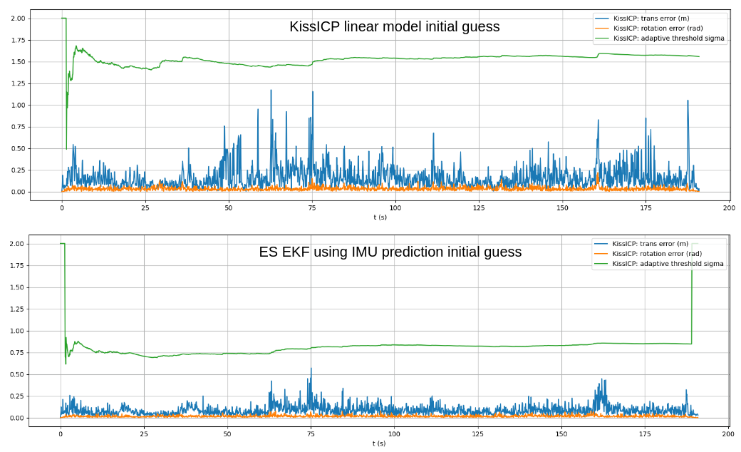
The full pipeline with Ouster Lidar data and its IMU data streams was implemented in the ptudes ekf-bench ouster command that accepts Ouster raw data recordings in pcap/bag formats. Additionally ground truth can be provided in Newer College Dataset format using --gt-file param which is used only to compare the results and compare the graphs of trajectories (using --plot graphs) and the adaptive threshold of the KissICP registration together with it’s corrected pose translation and rotation components (the less value of sigma of the adaptive threshold the more “confident” KissICP registration is for the particular scan, see [2] for KissICP algorithm details).
Tests was performed using sequences quad-easy/medium/hard and stairs from collection1 and park0, park1 and cloister0 from collection2, with/without using ES EKF imu prediction guess for KissICP registration. Additionally the tests with manually reduced beams number (32,64 and 128) on quad-medium sequence was compared. In majority of test cases the ES EKF imu predicted initial guess improved the resulting pose with reduced ATE errors, the most significant gains observed on 32 beams cases and harder movements like quad-hard or stairs sequences, see Table 1. for full results.
| Sequence name | Lidar Beams | KissICP range (m) min - max | ATE (deg) / trans (m) | ATE rot (deg) / trans (m) w imu prediction |
|---|---|---|---|---|
| nc-quad-easy | 128 | 1 - 35 | 0.0256 / 0.1383 | 0.0282 / 0.1834 |
| nc-quad-easy | 64 | 1 - 35 | 0.0318 / 0.0978 | 0.0791 / 0.8966 |
| nc-quad-easy | 32 | 1 - 35 | 1.0932 / 7.6802 | 0.3722 / 6.1207 |
| nc-quad-medium | 128 | 1 - 35 | 0.0715 / 0.3817 | 0.0434 / 0.1121 |
| nc-quad-medium | 64 | 1 - 35 | 0.1884 / 1.5852 | 0.2190 / 1.8996 |
| nc-quad-medium | 32 | 1 - 35 | 5.7766 / 36.7806 | 0.5252 / 6.1870 |
| nc-quad-hard | 128 | 1 - 35 | 0.1072 / 0.3465 | 0.0954 / 0.3582 |
| nc-quad-hard | 64 | 1 - 35 | 0.3947 / 5.5880 | 0.1045 / 0.3003 |
| nc-quad-hard | 32 | 1 - 35 | 1.8676 / 22.8112 | 0.3869 / 6.9918 |
| nc-stairs | 128 | 1 - 17 | 1.1885 / 0.3389 | 0.3467 / 0.1182 |
| nc-park0 | 128 | 1 - 35 | 0.5302 / 24.3595 | 0.5379 / 24.5963 |
| nc-park1 | 128 | 1 - 35 | 0.1151 / 8.3812 | 0.0593 / 2.4570 |
| nc-cloister0 | 128 | 1 - 17 | 0.3031 / 6.0323 | 0.3014 / 5.7621 |
| nc-cloister0 | 128 | 1 - 35 | 0.1598 / 2.9759 | 0.2001 / 3.8562 |
Table 1. Test results using ES EKF pipeline with IMU predicted initial guess vs linear KissICP initial guess (baseline).
The adaptive threshold value of KissICP tracks in most cases lower with IMU prediction pose guess (correspondingly the difference to corrected pose after ICP iterations is also lower), see Fig 3.
Source code and CLI to run it with Ouster Lidar sensors data
The ES EKF + KissICP trajectory smoothing developed as part of ptudes ekf-bench (Point eTudes) playground and can be installed from PyPi (python 3.7-3.11, Win/Mac/Linux supported):
pip install ptudes-lab
For example to run on the cloister0 sequence bag from Newer College Dataset and visualize the result you can run:
# process raw Ouster packets from .bag and run KissICP + ES EKF smoothing and save traj poses
ptudes ekf-bench ouster ./newer-college/2021-ouster-os0-128-alphasense/collection2/2021-12-02-10-15-59_0-cloister.bag \
  --save-nc-gt-poses cloister0-traj.csv

# visualize the part of the bag in a flyby tool
ptudes flyby ./newer-college/2021-ouster-os0-128-alphasense/collection2/2021-12-02-10-15-59_0-cloister.bag \
  --nc-gt-poses cloister0-traj.csv \
  --start-scan 400 \
  --end-scan 800
With the viz result shown below:
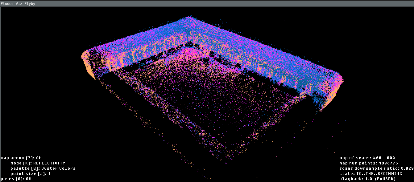
ptudes flyby over the cloister0 sequence scans 400-800Simulated IMU runs, ES EKF with real IMU topic but ground truth poses as a correction or comparing various trajectories with ATE scores calculated use ptudes ekf-bench sim, ptudes ekf-bench nc and ptudes ekf-bench cmp correspondingly.
To get the overall statistic of the IMU/Lidar scans from the pcap/bag you can use ptudes stat which may hint you the optimal value of --kiss-min-range/--kiss-max-range params to use:
ptudes stat ./newer-college/2021-ouster-os0-128-alphasense/collection2/2021-12-02-10-15-59_0-cloister.bag -t 0
With an output:
StreamStatsTracker[dt: 186.5307 s, imus: 18652, scans: 1866]:
  range_mean: 4.457 m,
  range_std: 4.139 m (s3 span: [0.234 - 16.874 m])
  range min max: 0.234 - 220.712 m
  acc_mean: [-0.18887646  0.41429864  9.72023424] m/s^2
  acc_std: [0.63840631 0.59747534 2.30738675]
  gyr_mean: [-0.01103721 -0.00591911  0.07017822] rad/s
  gyr_std: [0.09329166 0.14244756 0.34110766]
Gravity vector estimation:  [-0.01940998  0.0425756   0.99890469]
NOTE: estimated gravity vector doesn’t account for the movements and valid only when the lidar was stationary during the recording.
Checkout the previous blog post on (Point eTudes) for other nits.
Possible future work and experiments
ES EKF is a common building block in state-of-the art and recent efforts in Lidar Inertial Odometry like FAST-LIO2 [15], LIO-EKF [14], SR-LIO and many others. However, as mentioned above algorithms are tightly coupled LIO systems and they usually has much better performance than loosely-coupled counterparts, so it’s worth considering them for further adoption and experimenting to get the better Lidar-Inertial odometry.
References
- Lee, Dongjae, et al. “LiDAR Odometry Survey: Recent Advancements and Remaining Challenges.” (2023)
- Vizzo, Ignacio, et al. “Kiss-icp: In defense of point-to-point icp–simple, accurate, and robust registration if done the right way.” (2023)
- Ouster SDK: C++/Python sensor driver and tools, CLI, PointViz, etc. “GitHub”
- Zhang, Lintong, et al. “Multi-camera lidar inertial extension to the newer college dataset.” (2021).
- Ouster sensor raw sample data “Sensor Docs/Sample Data
- Sola, Joan. “Quaternion kinematics for the error-state Kalman filter.” (2017).
- Shin, Eun-Hwan. “Estimation techniques for low-cost inertial navigation.” (2005).
- Maley, James, and DEVCOM Army Research Laboratory. “A Modular Approach to Kalman Filter Design and Analysis.” (2021).
- Durrant-Whyte, Hugh. “Multi Sensor Data Fusion.” (2001).
- Eade, Ethan. “Lie groups for 2d and 3d transformations.” (2017).
- Sola, Joan, Jeremie Deray, and Dinesh Atchuthan. “A micro Lie theory for state estimation in robotics.” (2018).
- Daniel Lawrence Lu, “SE(3) constraints for robotics” (2021).
- Zhang, Zichao, and Davide Scaramuzza. “A tutorial on quantitative trajectory evaluation for visual (-inertial) odometry.” (2018).
- Wu, Yibin, et al. “Lio-ekf: High frequency lidar-inertial odometry using extended kalman filters.” (2023).
- Xu, Wei, et al. “Fast-lio2: Fast direct lidar-inertial odometry.” (2022).
- Yuan, Zikang, et al. “Sr-lio: Lidar-inertial odometry with sweep reconstruction.” (2022).