Localization is an essential task for augmented reality, robotics, and self-driving car applications. It’s crucial for a system to know the exact pose (location and orientation) of the agent to do visualization, navigation, prediction, and planning.

Baidu released its massive self-driving Apolloscape dataset in March and now has a couple of ongoing challenges for ECCV 2018 Workshop: Vision-based Navigation for Autonomous Driving conference:

Task 1: Vision-based fine-grained lane markings segmentation
Task 2: Self-localization on the fly
Task 3: 3D car instance understanding

I pick the self-localization problem and create the whole pipeline to localize a car which is based only on camera images.

This article covers the very beginning of the journey and includes the reading and visualization of the Apolloscape dataset for localization task. Implement PoseNet [2] architecture for monocular image pose prediction and visualize results. I use Python and Pytorch for the task.

NOTE: If you want to jump straight to the code here is the GitHub repo. It’s is still an ongoing work where I intend to implement Vidloc [7], Pose Graph Optimization [3,8] and Structure from Motion [9] pipelines for Apolloscape Dataset in the context of the localization task.

NOTE 2 (update Mar 12, 2019): Today I’m releasing the second part of my journey with Structure from Motion (SfM) pipeline and OpenGL visualization for Apolloscape ZPark Sample implemented on C++.

Apolloscape Dataset

Apolloscape dataset emerged from the Baidu effort in 2017 to collect enough data with the modern sensors that can be used for self-driving car research. Dataset provides camera images, poses, dense LIDAR point clouds, 3d semantic maps, 3d lane markings, 2d segmentation labels. Eventually, they plan to reach 200K images, captured on 20km roads covering 5 sites from 3 cities. Initial dataset was released in March 2018 and continuously updated for the ongoing ECCV challenges.

For the challenge purpose, Apolloscape provides separate archives for the self-localization task. You can download the small (4Gb) self-localization-examples ZPark from Self-Localization Dataset page.

I use ZPark sample dataset for almost everything in this article from visualization to PoseNet training.

Apolloscape Pytorch Dataset

For Pytorch I need to have a Dataset object that prepares and feeds the data to the loader and then to the model. I want to have a robust dataset class that can:

support stereo and mono images
support train/validation splits that came along with data or generate a new one
support pose normalization
support different pose representations (needed mainly for visualization and experiments with loss functions)
support filtering by record id
support general Apolloscape folder structure layout

I am not putting here the full listing of the Apolloscape dataset and concentrate solely on how to use it and what data we can get from it. For the full source code, please refer to the Github file datasets/apolloscape.py.

Here how to create a dataset:

from datasets.apolloscape import Apolloscape
from torchvision import transforms

# Path to unpacked data folders
APOLLO_PATH = "./data/apolloscape"

# Resize transform that is applied on every image read
transform = transforms.Compose([transforms.Resize(250)])

apollo_dataset = Apolloscape(root=os.path.join(APOLLO_PATH), road="zpark-sample",
                             transform=transform, train=True, pose_format='quat',
                             stereo=True)
print(apollo_dataset)

Output:

Dataset: Apolloscape
    Road: zpark-sample
    Record: None
    Train: None
    Normalize Poses: False
    Stereo: True
    Length: 1499 of 1499
    Cameras: ['Camera_2', 'Camera_1']
    Records: ['Record001', 'Record002', 'Record003', 'Record004', 'Record006', 'Record007', 'Record008', 'Record009', 'Record010', 'Record011', 'Record012', 'Record013', 'Record014']

APOLLO_PATH is a folder with unpacked Apolloscape datasets, e.g. $APOLLO_PATH/road02_seg or $APOLLO_PATH/zpark. Download data from Apolloscape page and unpack iot. Let’s assume that we’ve also created a symlink ./data/apolloscape that points to $APOLLO_PATH folder.

We can view the list of available records with a number of data samples in each:

# Show records with numbers of data points
recs_num = apollo_dataset.get_records_counts()
recs_num = sorted(recs_num.items(), key=lambda kv: kv[1], reverse=True)
print("Records:")
print("\n".join(["\t{} - {}".format(r[0], r[1]) for r in recs_num ]))

Output:

Records:
	Record008 - 122
	Record007 - 121
	Record006 - 121
	Record012 - 121
	Record001 - 121
	Record009 - 121
	Record010 - 121
	Record003 - 121
	Record013 - 120
	Record004 - 120
	Record002 - 120
	Record011 - 120
	Record014 - 50

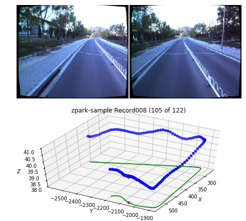
We can draw a route for one record with a sampled camera image:

from utils.common import draw_record

# Draw path of a record with a sampled datapoint
record = 'Record008'
draw_record(apollo_dataset, record)
plt.show()

Output:

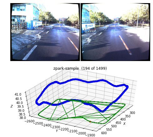
Record008 path and sampled stereo images pair (top). Blue - record path. Red - image pair location. Green - path projection on z-plane.

Alternatively, we can see all records at once in one chart:

# Draw all records for current dataset
draw_record(apollo_dataset)
plt.show()

Output:

All records from the dataset on one chart. Path projection connects the end of one record and the beginning of the next record.

Another option is to see it in a video:

from utils.common import make_video

# Generate and save video for the record
outfile = "./output_data/videos/video_{}_{}.mp4".format(apollo_dataset.road, apollo_dataset.record)
make_video(apollo_dataset, outfile=outfile)

Output (cut gif version of the generated video):

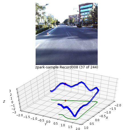
Generated video sample for Record008

For the PoseNet training we will use mono images with zero-mean normalized poses and camera images center-cropped to 250px:

# Resize and CenterCrop
transform = transforms.Compose([
    transforms.Resize(260),
    transforms.CenterCrop(250)
])

# Create train dataset with mono images, normalized poses, enabled cache_transform
train_dataset = Apolloscape(root=os.path.join(APOLLO_PATH), road="zpark-sample",
                             transform=transform, train=True, pose_format='quat',
                             normalize_poses=True, cache_transform=True,
                             stereo=False)

# Draw path of a single record (mono with normalized poses)
record = 'Record008'
draw_record(apollo_dataset, record)
plt.show()

Output:

Normalised poses and mono images resized and cropped to 250px.

Implemented Apolloscape Pytorch dataset also supports cache_transform option which is when enabled saves all transformed pickled images to a disk and retrieves it later for the subsequent epochs without the need to redo convert and transform operations every image read event. Cache saves up to 50% of the time during training time though it’s not working with image augmentation transforms like torchvision.transforms.ColorJitter.

Also, we can get the mean and the standard deviation that we need later to recover true poses translations:

poses_mean = train_dataset.poses_mean
poses_std = train_dataset.poses_std
print('Translation poses_mean = {} in meters'.format(poses_mean))
print('Translation poses_std  = {} in meters'.format(poses_std))

Output:

Translation poses_mean = [  449.95782055 -2251.24771214    40.17147932] in meters
Translation poses_std  = [123.39589457 252.42350964   0.28021513] in meters

You can find all mentioned examples in Apolloscape_View_Records.ipynb notebook.

And now let’s turn to something useful and more interesting, for example, training PoseNet deep convolutional network to regress poses from camera images.

PoseNet localization task

In general case, online localization task formulation goes like this: find the current robot pose $\mathbf{X}_t$ given its previous state $\mathbf{X}_{t-1}$ and current sensors observations $\mathbf{Z}_t$:

\[\mathbf{X}_t = f( \mathbf{X}_{t-1}, \mathbf{Z}_{t} )\]

PoseNet deep convolutional neural network regresses robot pose from monocular image; thus we are not taking in account previous robot state $\mathbf{X}_{t-1}$ at all:

\[\mathbf{X}_t = f( \mathbf{Z}_t )\]

Our observation sensor is a camera that gives us a monocular image $\mathbf{I}_t$. After removing subscript indexes for simplicity, we can define our task as to find a pose $\mathbf{X}$ given a monocular image $\mathbf{I}$.

\[\mathbf{X} = f( \mathbf{I} )\]

where $\mathbf{X}$ represents the full pose with translation $\mathbf{x}$ and rotation $\mathbf{q}$ components:

\[\mathbf{X} = [ \mathbf{x}, \mathbf{q} ] \\ \mathbf{x} = [x, y, z], \quad \mathbf{q} = [ q_1, q_2, q_3, q_4]\]

Rotation is represented in quaternions because they do not suffer from a wrap around $2\pi$ radians as Euler angles or axis-angle representations and more straightforward to deal than 3x3 rotation matrices.

For more information about the selection of different pose representation for deep learning refer to the excellent paper “Geometric loss functions for camera pose regression with deep learning” by Alex Kendall et al.

PoseNet Architecture

I build a DNN-based regressor for camera pose on ResNet and modify it by adding a global average pooling layer after the last convolutional layer and introducing a fully-connected layer with 2048 neurons. Finally, it’s concluded with 6 DoF camera pose regressor for translation $(x, y, z)$, and rotation $(q_1, q_2, q_3, q_4)$ vectors.

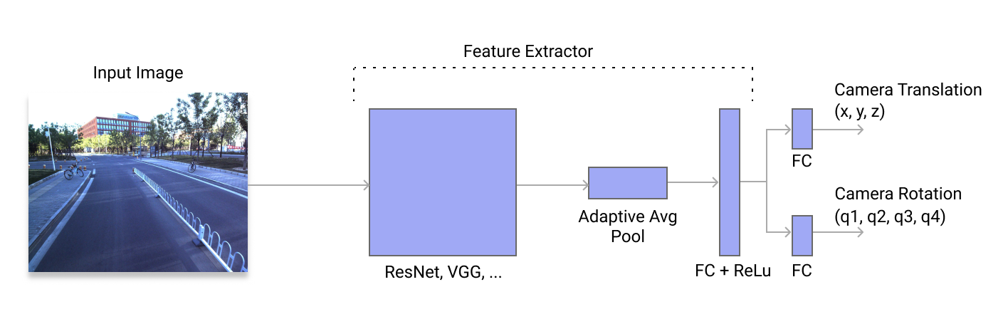
A PoseNet architecture with feature extractor network and regressors for camera translation and rotation. Feature extractor can be a pretrained on ImageNet ResNet18, ResNet34 or ResNet50.

A Pytorch implementation of the PoseNet model using a mono image:

import torch
import torch.nn.functional as F

class PoseNet(torch.nn.Module):

    def __init__(self, feature_extractor, num_features=128, dropout=0.5,
                 track_running_stats=False, pretrained=False):
        super(PoseNet, self).__init__()
        self.dropout = dropout
        self.feature_extractor = feature_extractor
        self.feature_extractor.avgpool = torch.nn.AdaptiveAvgPool2d(1)
        fc_in_features = self.feature_extractor.fc.in_features
        self.feature_extractor.fc = torch.nn.Linear(fc_in_features, num_features)

        # Translation
        self.fc_xyz = torch.nn.Linear(num_features, 3)

        # Rotation in quaternions
        self.fc_quat = torch.nn.Linear(num_features, 4)

    def extract_features(self, x):
        x_features = self.feature_extractor(x)
        x_features = F.relu(x_features)
        if self.dropout > 0:
            x_features = F.dropout(x_features, p=self.dropout, training=self.training)
        return x_features

    def forward(self, x):
        x_features = self.extract_features(x)
        x_translations = self.fc_xyz(x_features)
        x_rotations = self.fc_quat(x_features)
        x_poses = torch.cat((x_translations, x_rotations), dim=1)
        return x_poses

For further experiments I’ve also implemented stereo version (currently it’s simply processes two images in parallel without any additional constraints), option to switch off stats tracking for BatchNorm layers and Kaiming He normal for weight initialization [4]. Full source code is here models/posenet.py

PoseNet Loss Functions

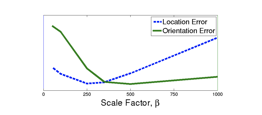
As a loss function I use a weighted combination of losses for translation and orientation as described in the original PoseNet paper [2]:

\[\mathcal{L}_{\beta} (\mathbf{I}) = \mathcal{L}_{x}(\mathbf{I}) + \beta \mathcal{L}_{q}(\mathbf{I})\]

Scaling factor $\beta$ was introduced to balance the losses of two variables expressed in different units and of different scales. Weighting param depends on the task itself and should be selected as a model hyper-parameter.

Example of parameter $ \beta $ influence on convnet performance on Chess scene from 7Scenes.
Source: Alex Kendall [2]

The second option for a loss function is to use a learning approach to find an optimal weighting for translation and orientation:

\[\mathcal{L}_{\sigma}(\mathbf{I}) = \frac{\mathcal{L}_x(\mathbf{I})}{\hat{\sigma}_x^2} + \log \hat{\sigma}_x^2 + \frac{\mathcal{L}_q(\mathbf{I})}{\hat{\sigma}_q^2} + \log \hat{\sigma}_q^2\]

$ \hat{\sigma}_x^2, \hat{\sigma}_q^2 $, homoscedastic uncertainties, represent free scalar values that we learn through backpropagation with respect to the loss function. Their effect is to decrease or increase the corresponding loss component automatically. And $ \log \hat{\sigma}_x^2, \log \hat{\sigma}_q^2 $ are the corresponding regularizers that prevent these values to become too big.

In practice, to prevent the potential division by zero, authors [1] suggest learning $ \hat{s} := \log \hat{\sigma}^2 $ which is more numerically stable. So the final loss expression looks like:

\[\mathcal{L}_{\sigma}(\mathbf{I}) = \mathcal{L}_x(\mathbf{I}) exp(-\hat{s}_{x}) + \hat{s}_{x} + \mathcal{L}_q(\mathbf{I}) exp(-\hat{s}_q) + \hat{s}_q\]

Initial values for $\hat{s}_{x}$ and $\hat{s}_q$ could be set via a best guess and I follow the suggestion from paper and set them to the values of $\hat{s}_{x} = 0, \hat{s}_q = -3.0$

For more details on where it came from and intro to Bayesian Deep Learning (BDL) you can refer to an excellent post by Alex Kendall where he explains different types of uncertainties and its implications to the multi-task models. And even more results you can find in papers “Multi-task learning using uncertainty to weigh losses for scene geometry and semantics.” [5] and “What uncertainties do we need in Bayesian deep learning for computer vision?.” [6].

Pytorch implementation for both versions of a loss function is the following:

class PoseNetCriterion(torch.nn.Module):
    def __init__(self, beta = 512.0, learn_beta=False, sx=0.0, sq=-3.0):
        super(PoseNetCriterion, self).__init__()
        self.loss_fn = torch.nn.L1Loss()
        self.learn_beta = learn_beta
        if not learn_beta:
            self.beta = beta
        else:
            self.beta = 1.0
        self.sx = torch.nn.Parameter(torch.Tensor([sx]), requires_grad=learn_beta)
        self.sq = torch.nn.Parameter(torch.Tensor([sq]), requires_grad=learn_beta)

    def forward(self, x, y):
        # Translation loss
        loss = torch.exp(-self.sx) * self.loss_fn(x[:, :3], y[:, :3])
        # Rotation loss
        loss += torch.exp(-self.sq) * self.beta * self.loss_fn(x[:, 3:], y[:, 3:]) + self.sq
        return loss

If learn_beta param is False it’s a simple weighted sum version of the loss and if learn_beta is True it’s using sx and sq params with enabled gradients that trains together with other network parameter with the same optimizer.

PoseNet Training Implementation Details

Now let’s combine it all to the training loop. I use torch.optim.Adam optimizer with learning rate 1e-5, ResNet34 pretrained on ImageNet as a feature extractor and 2048 features on the last FC layer before pose regressors.

from torchvision import transforms, models
import torch.optim as optim
from torch.utils.data import Dataset, DataLoader
from datasets.apolloscape import Apolloscape
from utils.common import save_checkpoint
from models.posenet import PoseNet, PoseNetCriterion

APOLLO_PATH = "./data/apolloscape"

# ImageNet normalization params because we are using pre-trained
# feature extractor
normalize = transforms.Normalize(mean=[0.485, 0.456, 0.406],
                                     std=[0.229, 0.224, 0.225])

# Resize data before using
transform = transforms.Compose([
    transforms.Resize(260),
    transforms.CenterCrop(250),
    transforms.ToTensor(),
    normalize
])

# Create datasets
train_dataset = Apolloscape(root=os.path.join(APOLLO_PATH), road="zpark-sample",
    transform=transform, normalize_poses=True, pose_format='quat', train=True, cache_transform=True, stereo=False)
val_dataset = Apolloscape(root=os.path.join(APOLLO_PATH), road="zpark-sample",
    transform=transform, normalize_poses=True, pose_format='quat', train=False, cache_transform=True, stereo=False)

# Dataloaders
train_dataloader = DataLoader(train_dataset, batch_size=80, shuffle=True)
val_dataloader = DataLoader(val_dataset, batch_size=80, shuffle=True)

# Select primary device
if torch.cuda.is_available():
    device = torch.device('cuda')
else:
    device = torch.device('cpu')

# Create pretrained feature extractor
feature_extractor = models.resnet34(pretrained=True)

# Num features for the last layer before pose regressor
num_features = 2048

# Create model
model = PoseNet(feature_extractor, num_features=num_features, pretrained=True)
model = model.to(device)

# Criterion
criterion = PoseNetCriterion(stereo=False, learn_beta=True)
criterion = criterion.to(device)

# Add all params for optimization
param_list = [{'params': model.parameters()}]
if criterion.learn_beta:
    # Add sx and sq from loss function to optimizer params
    param_list.append({'params': criterion.parameters()})

# Create optimizer
optimizer = optim.Adam(params=param_list, lr=1e-5, weight_decay=0.0005)

# Epochs to train
n_epochs = 2000

# Main training loop
val_freq = 200
for e in range(0, n_epochs):
    train(train_dataloader, model, criterion, optimizer, e, n_epochs, log_freq=0,
         poses_mean=train_dataset.poses_mean, poses_std=train_dataset.poses_std,
         stereo=False)
    if e % val_freq == 0:
        validate(val_dataloader, model, criterion, e, log_freq=0,
            stereo=False)

# Save checkpoint
save_checkpoint(model, optimizer, criterion, 'zpark_experiment', n_epochs)

A little bit simplified train function below with error calculation that is used solely for logging purposes:

def train(train_loader, model, criterion, optimizer, epoch, max_epoch,
          log_freq=1, print_sum=True, poses_mean=None, poses_std=None,
          stereo=True):

    # switch model to training
    model.train()

    losses = AverageMeter()

    epoch_time = time.time()

    gt_poses = np.empty((0, 7))
    pred_poses = np.empty((0, 7))

    end = time.time()
    for idx, (batch_images, batch_poses) in enumerate(train_loader):
        data_time = (time.time() - end)

        batch_images = batch_images.to(device)
        batch_poses = batch_poses.to(device)

        out = model(batch_images)
        loss = criterion(out, batch_poses)

        # Training step
        optimizer.zero_grad()
        loss.backward()
        optimizer.step()

        losses.update(loss.data[0], len(batch_images) * batch_images[0].size(0) if stereo
                else batch_images.size(0))

        # move data to cpu & numpy
        bp = batch_poses.detach().cpu().numpy()
        outp = out.detach().cpu().numpy()
        gt_poses = np.vstack((gt_poses, bp))
        pred_poses = np.vstack((pred_poses, outp))

        # Get final times
        batch_time = (time.time() - end)
        end = time.time()

        if log_freq != 0 and idx % log_freq == 0:
            print('Epoch: [{}/{}]\tBatch: [{}/{}]\t'
                  'Time: {batch_time:.3f}\t'
                  'Data Time: {data_time:.3f}\t'
                  'Loss: {losses.val:.3f}\t'
                  'Avg Loss: {losses.avg:.3f}\t'.format(
                   epoch, max_epoch - 1, idx, len(train_loader) - 1,
                   batch_time=batch_time, data_time=data_time, losses=losses))


    # un-normalize translation
    unnorm = (poses_mean is not None) and (poses_std is not None)
    if unnorm:
        gt_poses[:, :3] = gt_poses[:, :3] * poses_std + poses_mean
        pred_poses[:, :3] = pred_poses[:, :3] * poses_std + poses_mean

    # Translation error
    t_loss = np.asarray([np.linalg.norm(p - t) for p, t in zip(pred_poses[:, :3], gt_poses[:, :3])])

    # Rotation error
    q_loss = np.asarray([quaternion_angular_error(p, t) for p, t in zip(pred_poses[:, 3:], gt_poses[:, 3:])])

    if print_sum:
        print('Ep: [{}/{}]\tTrain Loss: {:.3f}\tTe: {:.3f}\tRe: {:.3f}\t Et: {:.2f}s\t{criterion_sx:.5f}:{criterion_sq:.5f}'.format(
            epoch, max_epoch - 1, losses.avg, np.mean(t_loss), np.mean(q_loss),
            (time.time() - epoch_time), criterion_sx=criterion.sx.data[0], criterion_sq=criterion.sq.data[0]))

validate function is similar to train except model.eval()/model.train() modes, logging and error calculations. Please refer to /utils/training.py on GitHub for full-versions of train and validate functions.

The training converges after about 1-2k epochs. On my machine, with GTX 1080 Ti it takes about 22 seconds per epoch on ZPark sample train dataset with 2242 images pre-processed and scaled to 250x250 pixels. Total training time – 6-12 hours

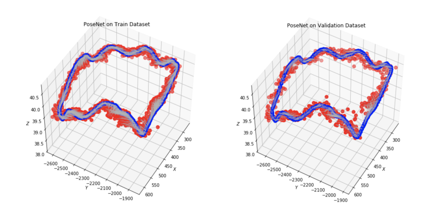
PoseNet training on ZPark sample road from Apolloscape dataset, 2k epochs and auto learn of scale factor for combined translation and rotation loss function. Te - translation error in meters. Re - rotation error in degrees.

PoseNet Results on Apolloscape dataset. ZPark sample road.

After 2k epochs of training, the model was managed to get a prediction of pose translation with a mean 40.6 meters and rotation with a mean 1.69 degrees.

Qualitative PoseNet model results after 2k epochs on train dataset (Left) and validation dataset (Right).

After learning, PoseNet criterion uncertainties became equal of $\hat{s}_{x} = 1.5606, \hat{s}_q = -3.8471$. Interestingly, these values are equivalent to the value of $\beta = 223.12$ which is close to those that can be derived from the PoseNet’ original paper [2].

Full PoseNet model, training and visualization code

You can replicate all results from this article using my GitHub repo of the project.

Further development

Established results are far from one that can be used in autonomous navigation where a system needs to now its location within accuracy of 15cm. Such precision is vital for a car to act safely, correctly predict the behaviors of others and plan actions accordingly. In any case, it’s a good baseline and building blocks of the pipeline to work with Apolloscape dataset that I can develop and improve further.

There many things to try next:

Use temporal nature of a video.
Rely on geometrical features of stereo cameras.
Pose graph optimization techniques.
Loss based on 3D reprojection errors.
Structure from motion methods to build 3D map representation.

And what’s more importantly, all above-mentioned methods need no additional information but that we already have in ZPark sample road from Apolloscape dataset.

References

Kendall, Alex, and Roberto Cipolla. “Geometric loss functions for camera pose regression with deep learning.” (2017).
Kendall, Alex, Matthew Grimes, and Roberto Cipolla. “Posenet: A convolutional network for real-time 6-dof camera relocalization.” (2015).
Brahmbhatt, Samarth, et al. “Mapnet: Geometry-aware learning of maps for camera localization.” (2017).
He, Kaiming, et al. “Delving deep into rectifiers: Surpassing human-level performance on imagenet classification.” (2015).
Kendall, Alex, Yarin Gal, and Roberto Cipolla. “Multi-task learning using uncertainty to weigh losses for scene geometry and semantics.” (2017).
Kendall, Alex, and Yarin Gal. “What uncertainties do we need in bayesian deep learning for computer vision?.” (2017).
Clark, Ronald, et al. “VidLoc: A deep spatio-temporal model for 6-dof video-clip relocalization.” (2017).
Calafiore, Giuseppe, Luca Carlone, and Frank Dellaert. “Pose graph optimization in the complex domain: Lagrangian duality, conditions for zero duality gap, and optimal solutions.” (2015).
Martinec, Daniel, and Tomas Pajdla. “Robust rotation and translation estimation in multiview reconstruction.” (2007).