Last year at CVPR 2018, I became interested in the Apolloscape dataset and the localization task challenge that was announced for ECCV 2018. I dived into the problem: exploring the Apolloscape dataset and using PoseNet with geometric loss functions [1,2] for direct pose prediction from monocular images. As a result, I got more interested in geometric approaches and multi-view geometry for computer vision tasks.

While direct deep-learning methods somewhat works for 6DOF pose regression, they are not yet precise, and research papers increasingly use a combination of the following methods: Structure from Motion (SfM) techniques, geometric-based constraints, pose graph optimizations [15] and 3D maps for scene understanding, visual odometry, and SLAM tasks.

In this project, I explore the traditional SfM pipeline and build sparse 3D reconstruction from the Apolloscape ZPark sample dataset with simultaneous OpenGL visualization.

My primary goal was to learn from the first principles and implement the pipeline myself. To make SfM in production or research, you might look into available libraries: COLMAP [3,4], MVE [5], openMVG [6], VisualSFM [7], PMVS2/CMVS [9] and Bundler [8].

In this text, I use words like image, camera, or view interchangeably to relate to the same concept of an image taken with a camera in a particular location (e.g., view), and it almost always means the same in my writing and code. Sometimes it’s an image when I am preparing a dataset; a camera when I calculate the distance or projective matrix; and a view when I am processing 3D maps and merging 3D points of different maps.

NOTE: Code with build instructions and a reconstructed 3D map example available in my GitHub repo.

Apolloscape Dataset

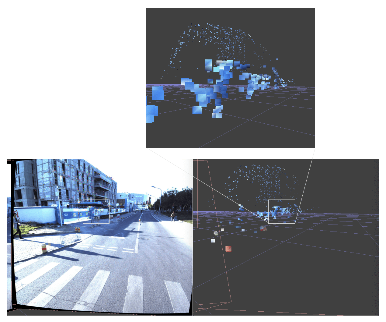
In my previous article, I visualize and explore the dataset. Here is the typical record (one of 13 for the ZPark sample):

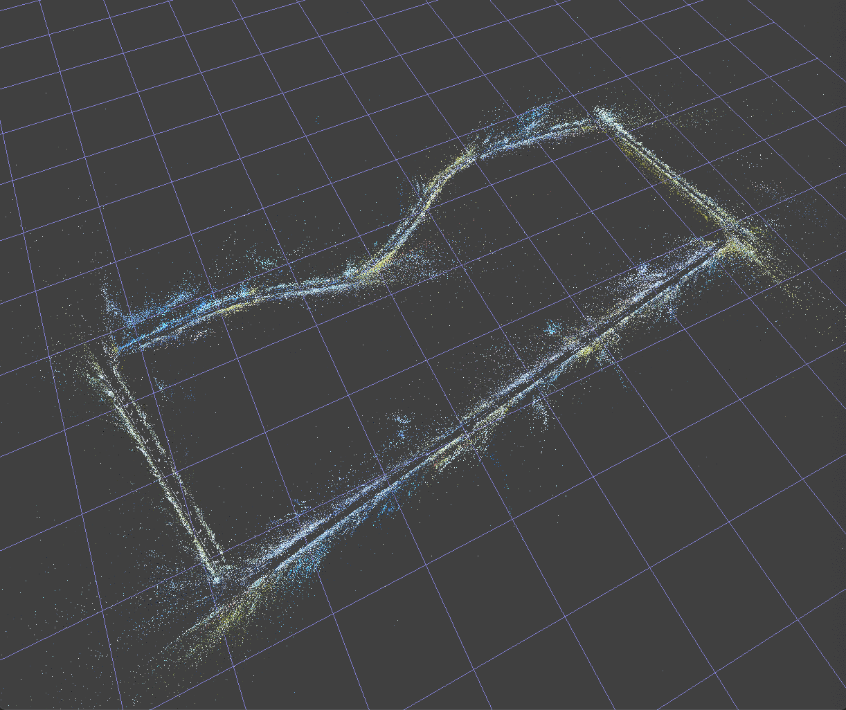
Here is an SfM 3D reconstruction obtained from the corner shown above on a video piece:

3D Reconstruction Results

In total, there 1,499 image pairs spread across 13 records in the Apolloscape ZPark sample dataset.

And below is the description of the behind the scenes SfM process.

SfM pipeline

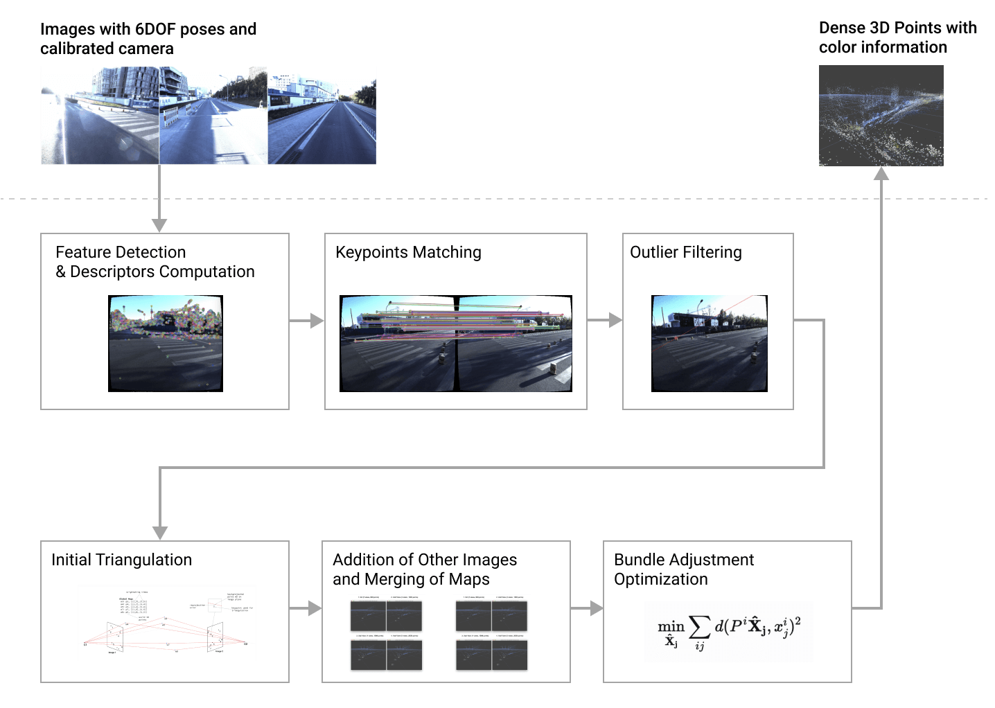
The 3D reconstruction process consists of 6 major steps:

1. Features Detection & Descriptors Computation
2. Keypoints Matching (make image pairs, match keypoints)
3. Outlier Filtering (via epipolar constraint)
4. Initial Triangulation (triangulation of the best image pair)
5. Addition of Other Images and Merging of Maps
6. Bundle Adjustment Optimization

The described pipeline doesn’t include a couple steps from traditional SfM because we already know camera poses and need to find only world-map 3D points. These additional steps are:

• 2D-3D matching – finds the correspondance of 2d keypoints with already calculated 3d points, however there part of it when we find the next best view to use
• New image registration – estimates projection matrices based on 2d-3d matches from the previous steps
• Camera pose calculation – finds camera translation and rotation from the projection matrix
• Bundle adjustment for camera poses, together with 3D map points.

The above parts can be easily added to the existing structure later when, and if, the need arises.

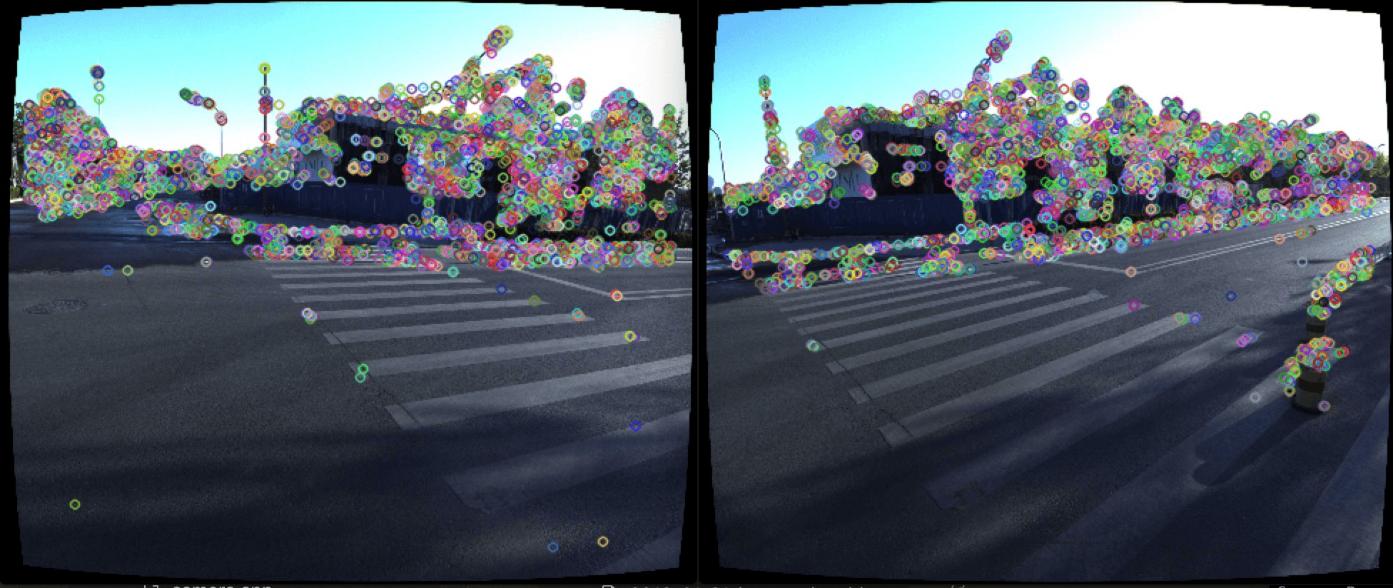
Features Detection & Descriptors Computation

First, we need to have distinctive points in the image for which we can compare and establish relationships in order to estimate image transformations or, as in the current task of reconstruction, to estimate their location in the space using multiple images.

There are lots of known reliable feature detectors: SURF, SIFT, ORB, BRISK, and AKAZE. I tried a couple of them from OpenCV and decided to stick with AKAZE, which gave enough points in a reasonable amount of time, with fast descriptor matching.

For further in-depth information about how different feature detectors compare, I recommend “A comparative analysis of SIFT, SURF, KAZE, AKAZE, ORB, and BRISK” [10].

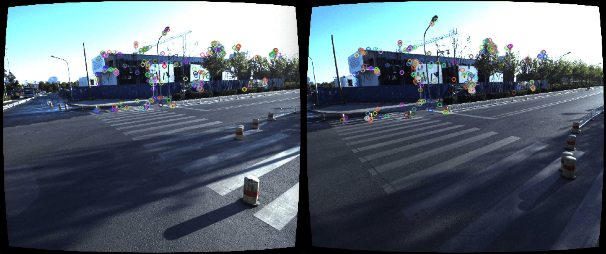
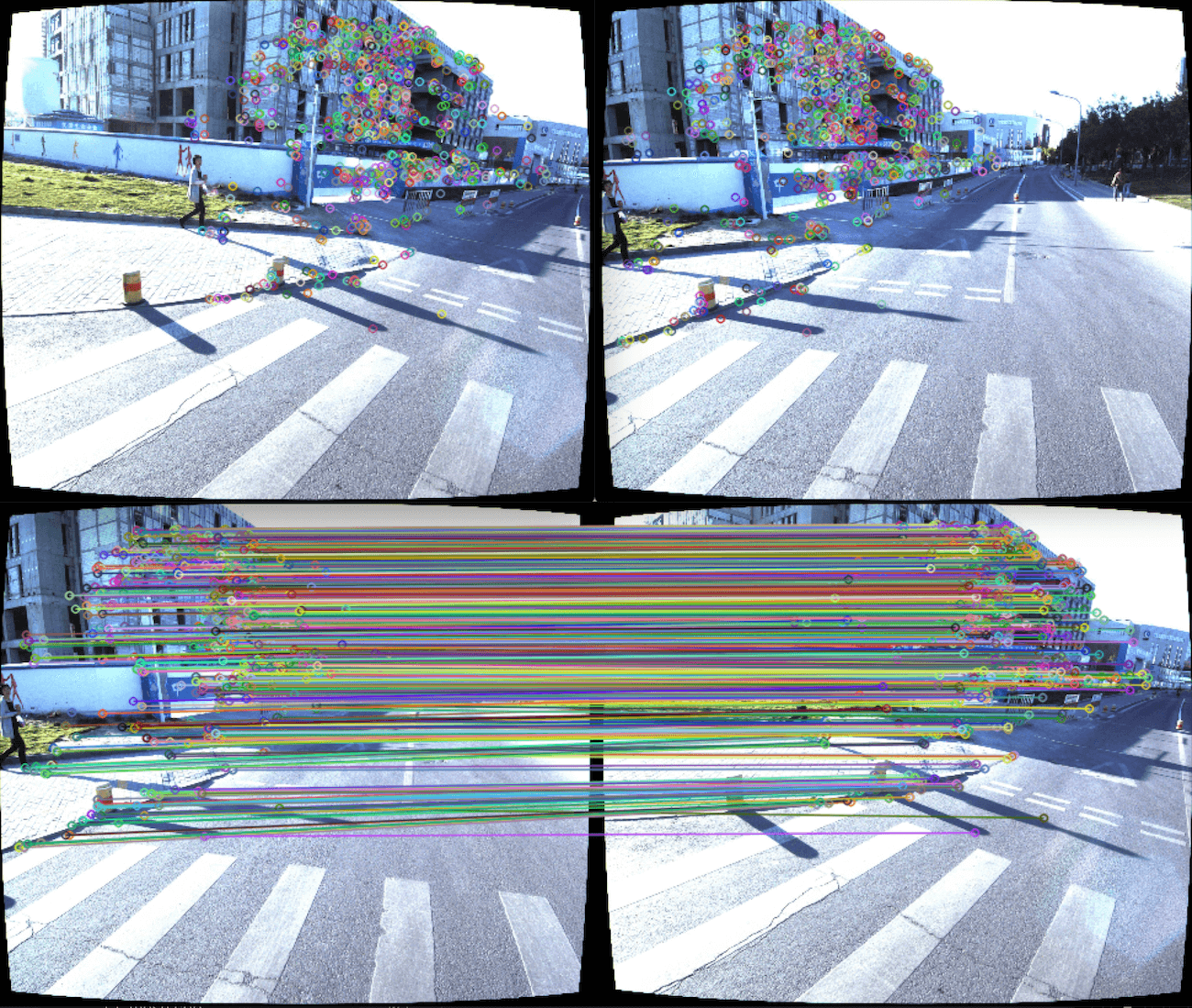
Keypoints Matching

The next step is to find the keypoints correspondence for every image pair. One of the common methods is to find two closest neighbors per point and compare the distance between them, aka Lowe’s ratio test [11]. If two closest neighbor points are located at the same distance from the original point, and they are not distinctive enough, we can skip the keypoint completely. Lowe’s paper concludes that ratio of 0.7 is a good predictor; however, in this case, I selected a ratio of 0.5 because it seemed to work better.

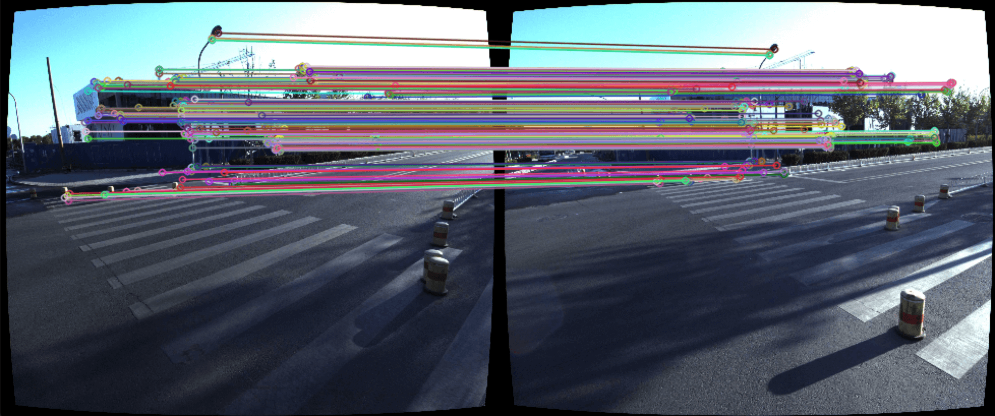
An additional test for keypoint correspondence is the epipolar constraint, which can be applied by having camera poses and computed fundamental matrix between two cameras. So I checked the distance between keypoints and the correspondent epipolar line, and then filtered the keypoints with a distance larger than threshold values (default is 10px).

The last step is to filter image pairs that have the small number of matched keypoints remaining after Lowe’s ratio test and epipolar constraint filtering. I set the value to seven matched points for small reconstructions (up to 200 images) and approximately 60 points for reconstructions with more than 1000 images.

Another important consideration was how to make image pairs for keypoints matching. The easiest way is to generate all pairs, but it takes too long to match the features for all image combinations. We can instead reduce the number of pairs because we know camera locations and thus include only pairs with cameras that are located nearby.

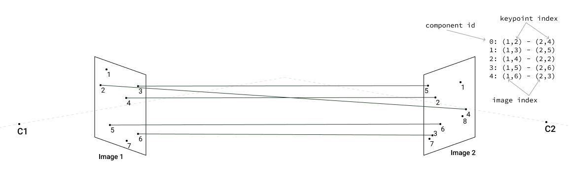
After we extract keypoints from images and match image pairs, we create a connected components graph to quickly find images with the most common connections. Here is an example of building connected components for three images.

First, we have one image pair [1,2]:

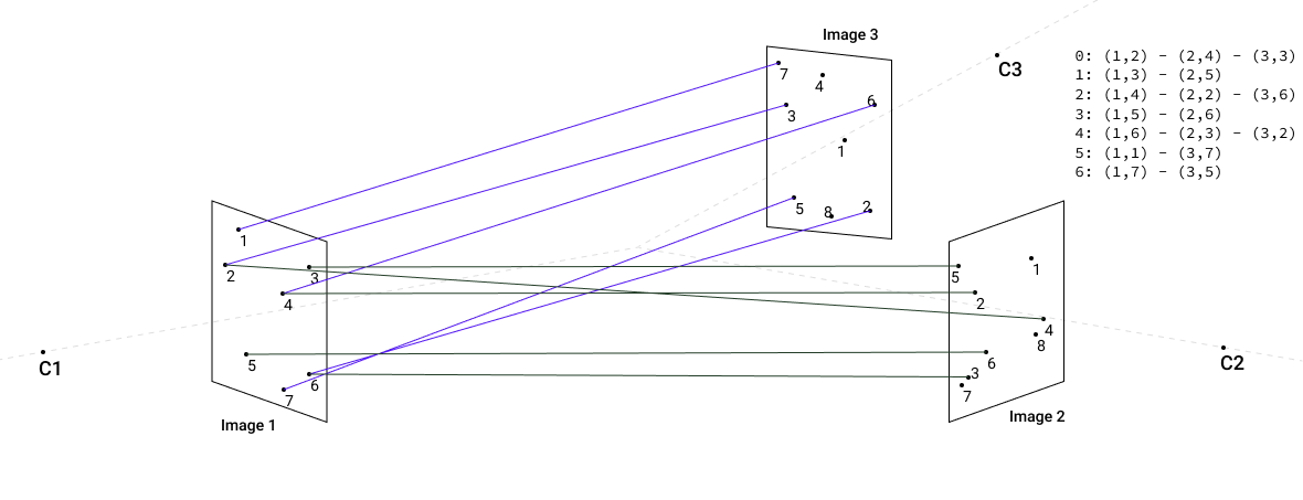
Then we add image pair [1,3] and continue connecting keypoints into components:

And finally we add matches for third image pair [2,3]:

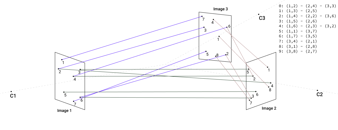
Internally connected components are implemented as a tree, with the balanced depth of the subtrees, in order to support fast find and union operation. Fast check for connectedness is important in the merge-maps step, when we need to check whether points belong to the same component and therefore can be merged.

Initial Triangulation

The best image pair is the one with the most matched keypoints, so we can use it for the initial triangulation step. The more keypoints we have from the first image pair in the reconstruction, the greater the chance that we will have to connect corresponding 3D points from different image pairs in subsequent steps.

It’s also important to have connected points because Bundle Adjustment Optimization will tie different point clouds together and minimize re-projection errors from the same 3D point on multiple images.

Linear triangulation is implememnted using the classical DLT methods described in Hartley/Zisserman (12.2 p312) [12] which describes finding a solution for the system of equations Ax=0 via SVD decomposition and taking the vector with the smallest singular value. For this purpose I used OpenCV function cv::triangulatePoints which is a pure SVD-based method.

For every 3D point, we are storing the list of both views and keypoints used to reconstruct this point.

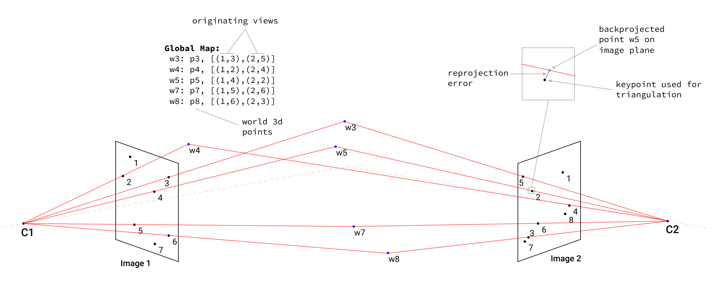
Initial reconstruction step in 3D visualization, with filtered outliers and Bundle Adjustment Optimization that further minimizes the re-projection error of the survived points.

Adding of Other Images and Merging of Maps

We then check the most connected image from the list of unprocessed views against the list of the views that were already used for reconstruction. Next, we iterate the previous step until all views are used. Finally, we triangulate the corresponding pairs to obtain the local point cloud.

Then local point clouds are merged into the global map along the points that belong to the same connected component, if the distance between two connected points lies within the threshold of 3.0m (hyperparameter).

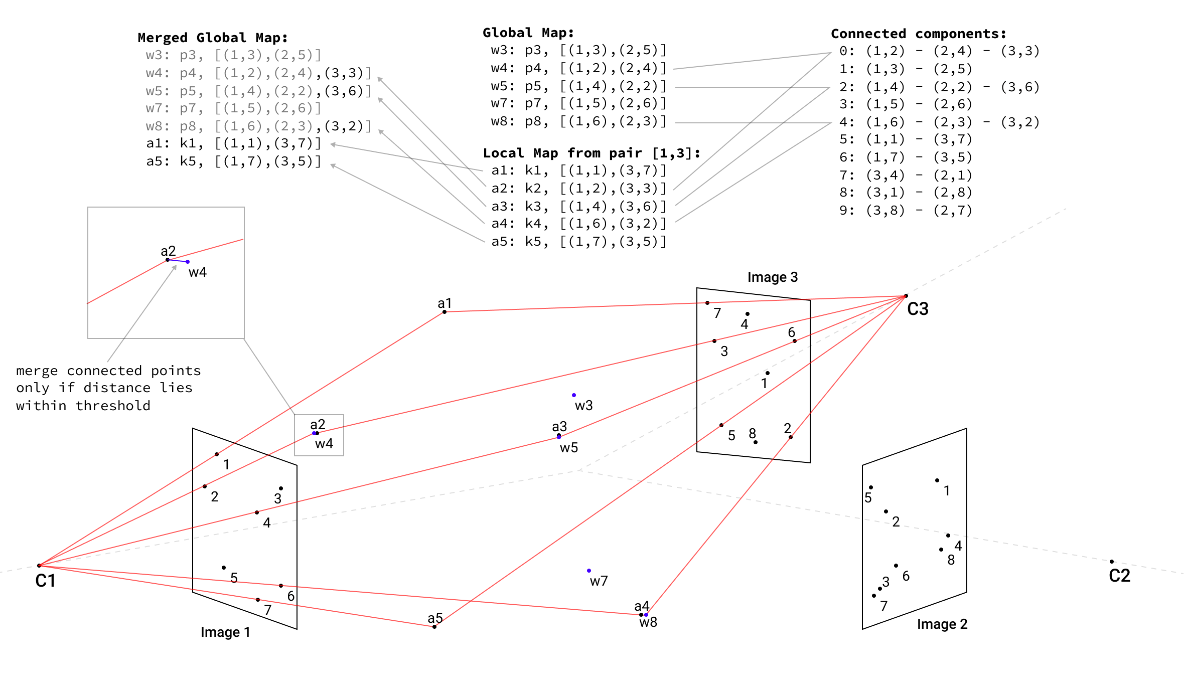
If the distance between connected points is bigger than the threshold, we discard both points from the map. Distinctive points without a connected points counterpart are copied to the global map without changes.

Below is an example of three subsequent steps after the initial reconstruction and its 3D visualization.

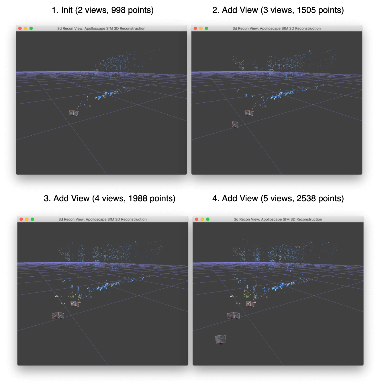
Thus we are increasing the resulting map with more and more 3D points while processing additional views.

Bundle Adjustment Optimization

After every step of merging the map and increasing the views list of 3D points, we can perform map optimization and jointly minimize the re-projection error for every point on every originating view.

Mathematically, the problem statement is to minimize the loss function:

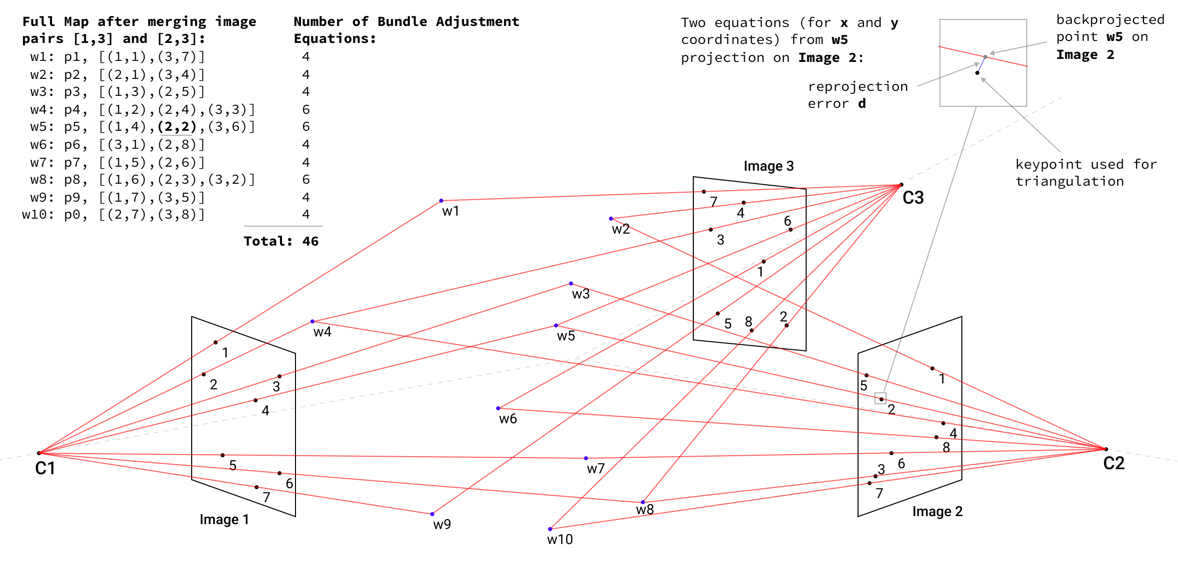
\[\min_{\mathbf{\hat{X}_j}} \sum_{ij} d(P^i \mathbf{\hat{X}_j}, x_j^i)^2\]

where \(d(a, b)\) is the geometric distance between two points; \(\mathbf{\hat{X}_j}\) is an estimated 3D point in a world space; \(P^i\) is a projection matrix for camera \(i\), \(x_j^i\) is 2D coordinates of a keypoint in image \(i\) that corresponds to the 3D point \(\mathbf{\hat{X}_j}\) and \(P^i \mathbf{\hat{X}_j}\) is a backprojection of point \(\mathbf{\hat{X}_j}\) to image \(i\).

I need to mention that this is a simpler formulation than usually encountered in full SLAM problems because we are not optimizing camera projection matrix \(P^i\) here (It’s known in the Apolloscape dataset). Furthermore, there is also no weighted matrix that accounts for variances in error contributions between different world points.

Below, we continue the reconstruction of our three image examples with the resulting merged map of ten 3D points that correspond to 46 equations in the Bundle Adjustment Optimization problem.

Without camera poses computation, as in a full SLAM problem, we set only 3D map points as parameters to the Ceres solver, which performs Non-linear Least Squares optimization using the Levenberg-Marquardt method.

Ceres solver was optimized to work with huge problems, so the optimizations of 1.4M 3D points is not too large for the library to handle (though it is demanding for CPU computation on my MacBook Pro:)

In order to save computation time, I run a Bundle Adjustment Optimization with Ceres solver only after I merge 40k new 3D points to the global map. Such a sparse optimization approach works because the problem is a constraint in just 3D map-point optimization with known camera poses, and thus is more or less localized in the parameter space. There also no such events like loop closures, as in SLAM problems, which might wreak havoc on the map without a proper optimization of the current graph reconstruction.

Visualization

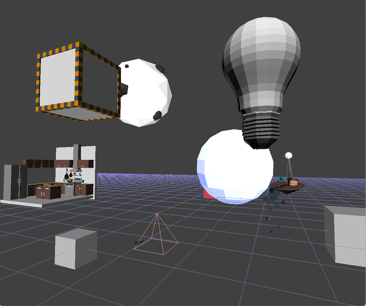
I visualize the 3D map, cameras, images, and back-projection points with OpenGL using GLFW, glad, glm and OpenCV for key-points visualization. The idea behind is to have camera parameters for OpenGL visualization identical to camera parameters of the dataset; this provides more intuition in multi-view projective geometry to allow for the exploration of the scene reconstruction, camera projections, and locations in one environment.

Everything in visualization is done with vertices, vertex array buffers, vertex/fragment/geometry shaders, and ambient and diffuse lightning. In addition, the functionality to load arbitrary 3D objects from common file formats (.obj, .fbx via assimp library) is helpful as visual clues for some experiments.

As for 3D points visualization, we can add color information estimated from keypoint vertices. Every point represented as a square with four distinctive colors on the vertices as a texture. Vertex colors are estimated as the average colors extracted from pixels of the corresponding vertices for every connected keypoint, adjusted to the rotation angle and the size of the keypoints.

This method provides a good understanding of keypoints and the region from which they were extracted (building, tree, road, etc.). However, many possible improvements can be done, for example, to add a center color point or to extract colors from the corresponding scaled version of the image. These methods allow for various keypoints octave and the visualization of squares in different sizes that account for variations in keypoint size.

Conclusion

SfM is a classical pipeline that is still widely used in SLAM, Visual Odometry, and Localization approaches.

Having completed this project, I can now much better appreciate the challenges of common computer vision problems, their algorithmic and computational complexities, the difficulty of getting 3D space back from the 2D images, as well as the importance of visualization tools and intuition in understanding algorithms that form the basis of software in AR glasses, VR headsets, and self-driving robots.

While finishing this write up, I discovered the new Localization challenge for CVPR 2019 as part of the workshop “Long-Term Visual Localization under Changing Conditions”. You can learn more at visuallocalization.net [16]

Yep, seems like I’ve found a new interesting problem and open datasets to play with for my next side project :)

References

1. Kendall, Alex, and Roberto Cipolla. “Geometric loss functions for camera pose regression with deep learning.” (2017).
2. Kendall, Alex, Matthew Grimes, and Roberto Cipolla. “Posenet: A convolutional network for real-time 6-dof camera relocalization.” (2015).
3. Schonberger, Johannes L., and Jan-Michael Frahm. “Structure-from-motion revisited.” (2016).
4. COLMAP: general-purpose Structure-from-Motion (SfM) and Multi-View Stereo (MVS) pipeline with a graphical and command-line interface. Project Page (2016).
5. MVE: an implementation of a complete end-to-end pipeline for image-based geometry reconstruction. Project Page
6. openMVG: “open Multiple View Geometry” Project Page
7. VisualSFM : A Visual Structure from Motion System Project Page
8. Bundler: Structure from Motion (SfM) for Unordered Image Collections Project Page
9. PMVS2: Patch-based Multi-view Stereo Software (PMVS - Version 2) PMVS2 Project Page & CMVS Project Page
10. Tareen, Shaharyar Ahmed Khan, and Zahra Saleem. “A comparative analysis of sift, surf, kaze, akaze, orb, and brisk.” (2018).
11. Lowe, David G. “Distinctive image features from scale-invariant keypoints.” (2004).
12. Hartley, Richard, and Andrew Zisserman. “Multiple view geometry in computer vision” (2003).
13. Alcantarilla, Pablo F., and T. Solutions. “Fast explicit diffusion for accelerated features in nonlinear scale spaces.” (2011)
14. Learn OpenGL - Modern OpenGL tutorial https://learnopengl.com/
15. Brahmbhatt, Samarth, et al. “Mapnet: Geometry-aware learning of maps for camera localization.” (2017).
16. Sattler, Torsten, et al. “Benchmarking 6dof outdoor visual localization in changing conditions.” (2018).